Hongyuan Huang

"\x48\x48\x59\x26\x48\x58\x59\x3A\x44"

All posts in one long list


Modern C++ Tutorials #7: Parallelism and Concurrency

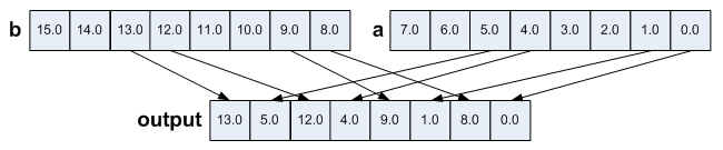
07 Parallelism and Concurrency

mutex and lock

  • std::lock_guard: RAII lock
  • std::unique_lock: similar to std::lock_guard with support for manual locking and unlocking, also used for locking std::shared_mutex when writing
  • std::shared_lock: provides concurrent reading of shared resource, must be used on a std::shared_mutex object

std::future

An asynchronous operation (created via std::async, std::packaged_task, or std::promise) can provide a std::future object to the creator of that asynchronous operation.

std::packaged_task is used when you have a callable that needs to be executed asynchronously and you want to obtain its result later.

packaged_task<int()> task( [](){
    this_thread::sleep_for(chrono::seconds(1)); 
    return 7;
} );
auto f = task.get_future();
thread worker(move(task));
worker.join();
cout << "You can see this immediately!\n";
f.get(); //block
cout << "You can see this after a second\n";

std::async is just a function template that creates and runs a std::packaged_task asynchronously. Think of it as an enhancement to std::thread which allows you to get the result back from another thread.

auto f = async( launch::async, [](){
    this_thread::sleep_for(chrono::seconds(1)); 
    return 7;
} );
cout << "You can see this immediately!\n";
f.get(); //block
cout << "This will be shown after a second!\n";

Note that std::async’s returned future will block upon destruction:

auto test_async() {
    auto f = async( launch::async, [](){
        this_thread::sleep_for(chrono::seconds(1)); 
        return 7;
    } );
    // future::~future() will block
    return f;
}

int main() {
    test_async(); //block
    cout << "This will be shown after a second!\n";

    auto f = test_async(); //non-block
    cout << "You can see this immediately !\n";
    f.get(); //block
    cout << "This will be shown after a second!\n";
    return 0;
}

std::promise is a class template that allows a value or an exception to be shared between threads.

promise<int> p;
auto f = p.get_future();
thread( [&p]{ 
    this_thread::sleep_for(chrono::seconds(1)); 
    p.set_value_at_thread_exit(9);
} ).detach();
f.get(); //block
cout << "This will be shown after a second!\n";

Relationship of std::async, std::packaged_task and std::promise? See this StackOverflow answer.

  • std::async is the most convenient and straight-forward way to perform an asynchronous com­pu­ta­tion is via the async function template, which returns the future. We have very little control over the details. In particular, we don’t even know if the function is exe­cu­ted concurrently, serially upon get(), or by some other black magic.
  • std::packaged_task can implement something like std::async, but in a fashion that we control.
  • std::promise is the lowest level of the implementation. The principal steps are these:
    • The calling thread makes a promise.
    • The calling thread obtains a future from the promise.
    • The promise, along with function arguments, are moved into a separate thread.
    • The new thread executes the function and fulfills the promise.
    • The original thread retrieves the result.

condition_variable

To use condition_variable properly, mutex and a predicate are both needed:

std::mutex mtx;
std::condition_variable cv; 
bool dataReady{false};

void waitingForWork(){
    std::cout << "Waiting " << std::endl;
    // condition_variable::wait() only accept unique_lock
    // acquire lock for reading
    std::unique_lock<std::mutex> lck(mtx);
    // release lock when waiting
    cv.wait(lck, []{ return dataReady; });
    // acquire lock again when awaken
    std::cout << "Running " << std::endl;
}

void setDataReady(){
    {
        // acquire lock for writing
        // prevent potential deadlock caused by missed signal
        std::lock_guard<std::mutex> lck(mtx);  
        dataReady = true;
    }
    std::cout << "Data prepared" << std::endl;
    // notification can be done outside of the lock
    cv.notify_one();
}

Here’s an example that would cause deadlock if cv.notify_one() is called before cv.wait().

It won’t happen in the first example because when cv.notify_one() is called, dataReady is guaranteed to be true so cv.wait() won’t block.

std::mutex mtx;
std::condition_variable cv;

void waitingForWork(){
    std::cout << "Waiting " << std::endl;
    std::unique_lock<std::mutex> lck(mtx);
    cv.wait(lck);
    std::cout << "Running " << std::endl;
}

void setDataReady(){
    std::cout << "Data prepared" << std::endl;
    cv.notify_one();
}

Another example that could also cause deadlock:

std::mutex mtx;
std::condition_variable cv;
std::atomic<bool> dataReady{false};

void waitingForWork(){
    std::cout << "Waiting " << std::endl;
    std::unique_lock<std::mutex> lck(mtx);
    cv.wait(lck, []{ return dataReady.load(); });
    std::cout << "Running " << std::endl;
}

void setDataReady(){
    dataReady = true;
    std::cout << "Data prepared" << std::endl;
    cv.notify_one();
}

Although unlikely, deadlock could occur when the code is executed in this order:

  • return dataReady.load(); // false
  • dataReady = true;
  • cv.notify_one();
  • cv.wait();

This can be observed easily by making the below modification to the code:

std::mutex mtx;
std::condition_variable cv;
std::atomic<bool> dataReady{false};

void waitingForWork(){
    std::cout << "Waiting " << std::endl;
    std::unique_lock<std::mutex> lck(mtx);
    cv.wait(lck, []{ 
        bool tmp = dataReady.load();
        std::this_thread::sleep_for(std::chrono::seconds(2)); 
        return tmp;
    });
    std::cout << "Running " << std::endl;
}

void setDataReady(){
    std::this_thread::sleep_for(std::chrono::seconds(1)); 
    dataReady = true;
    std::cout << "Data prepared" << std::endl;
    cv.notify_one();
}

std:atomic

int data = 0;
std::atomic<int> flag = {0};

std::thread release( [&]() {
    assert( data == 0 );
    data = 1;
    flag.store( 1, std::memory_order_release );
} );

std::thread acqrel( [&]() {
    int expected = 1;
    while( !flag.compare_exchange_strong( expected, 2, std::memory_order_acq_rel ) ) {
        assert( expected == 0 );
        expected = 1;
    }
} );

std::thread acquire( [&]() {
    while( flag.load(std::memory_order_acquire) < 2 );
    assert( data == 1 );
} );

release.join();
acqrel.join();
acquire.join();

Modern C++ Tutorials #4: Containers

04 Containers

std::array

With a std::array, the element type and array length are part of the type information.

// Doesn't work:
// void printArray(const std::array& myArray);
// OK but limited use case:
// void printArray(const std::array<int, 5>& myArray);

template <typename T, std::size_t size>
void printArray(const std::array<T, size>& myArray)
{
    for (auto element : myArray)
        std::cout << element << ' ';
    std::cout << '\n';
}

Modern C++ Tutorials #3: Language Runtime Enhancement

03 Language Runtime Enhancement

std::function

int foo(function<int( void )> lambda) {
    return lambda();
}

int main() {
    function<int( function<int( void )> )> bar = foo;
    cout << bar( [](){ return 100; } ) << endl;
    return 0;
}

std::bind and std::placeholder

int foo(int a, int b, int c) {
    return a * b + c;
}

int main() {
    auto bindFoo = bind(foo, placeholders::_1, 1, 2);
    cout << bindFoo(1) << endl;
}

lvalue, rvalue, prvalue, xrvalue

  • lvalue, left value, as the name implies, is the value to the left of the assignment symbol. To be precise, an lvalue is a persistent object that still exists after an expression (not necessarily an assignment expression).
  • rvalue, right value, the value on the right refers to the temporary object that no longer exists after the expression ends.
  • pvalue, pure rvalue, purely rvalue, either purely literal, such as 10, true; either the result of the evaluation is equivalent to a literal or anonymous temporary object, for example 1+2. Temporary variables returned by non-references, temporary variables generated by operation expressions, original literals, and Lambda expressions are all pure rvalue values.
  • xvalue, expiring value is the concept proposed by C++11 to introduce rvalue references (so in traditional C++, pure rvalue and rvalue are the same concepts), a value that is destroyed but can be moved.

rvalue reference and lvalue reference

  • lvalue ref & is a reference that binds to an lvalue (persistent).
  • rvalue ref && is a reference that binds to an rvalue (temporary).
  • lvalue ref can’t bind to rvalue.
  • const lvalue ref can bind to rvalue, it extends the lifetime of the temporary object and the object can’t be modified.
  • rvalue ref can bind to rvalue, it extends the lifetime of the temporary object and the object can be modified.

rvalue ref itself is a lvalue, because it has a name and can be referenced by its address:

void reference(int& v) {
    cout << "lvalue" << endl;
}
void reference(int&& v) {
    cout << "rvalue" << endl;
}
int main() {
    reference(1);       // prints "rvalue"
    auto&& a = 1;
    reference(a);       // prints "lvalue" because a is an lvalue
    reference(move(a)); // prints "rvalue"
    return 0;
}

Why not allow non-constant references to bind to non-lvalues? This is because there is a logic error in this approach:

void increase(int & v) {
    v++;
}
void foo() {
    double s = 1;
    increase(s); // s is converted to a temp int object, modifying the temp object won't change s
}

Why do constant references allow binding to non-lvalues? The reason is simple because Fortran needs it.

Some brain teasers:

int sourceArray[5] = {1, 2, 3, 4, 5};
int* destinationArray = move(sourceArray); // same as static_cast<int*>(sourceArray)
sourceArray[0] = 10;
cout << destinationArray[0] << endl;       // 10
/* Note that a literal (except a string literal) is a prvalue. 
 * However, a string literal is an lvalue with type const char array. 
 */
// Assert success. It is a const char [6] indeed. Note that decltype(expr)
// yields lvalue reference if expr is an lvalue and neither an unparenthesized
// id-expression nor an unparenthesized class member access expression.
static_assert(std::is_same<decltype("01234"), const char(&)[6]>::value, "");
 
// Correct. The type of "01234" is const char [6], so it is an lvalue
const char (&left)[6] = "01234";
// Error. "01234" is an lvalue, which cannot be referenced by an rvalue reference
// const char (&&right)[6] = "01234";
// Correct. std::move unconditionally convert lvalue to rvalue
const char (&&right)[6] = std::move("01234");

/* However, an array can be implicitly converted to a corresponding pointer.
 * The result, if not an lvalue reference, is an rvalue (xvalue if the result is an rvalue reference, prvalue otherwise)
 */
const char*   p      = "01234";   // Correct. "01234" is implicitly converted to const char*
const char* (&&pr)   = "01234";   // Correct. "01234" is implicitly converted to const char*, which is a prvalue
// const char* (&pl) = "01234";   // Error: lvalue can't ref to temp variable 
const char* const (&pl) = "1234"; // Correct: const lvalue reference can extend temp variable's lifecycle
void reference(string& str) {
    cout << "lvalue" << endl;
}
void reference(string&& str) {
    cout << "rvalue" << endl;
}

int main()
{
    string  lv1 = "string,";       // lv1 is a lvalue
    // string&& r1 = lv1;          // illegal, rvalue can't ref to lvalue
    string&& rv1 = move(lv1);      // legal, move can convert lvalue to rvalue
    cout << rv1 << endl;           // string,

    // string& l2 = lv1 + lv1;     // illegal, lvalue can't ref to temp variable 
                                   // (lv1 + lv1) is a temp variable

    const string& lv2 = lv1 + lv1; // legal, const lvalue reference can
                                   // extend temp variable's lifecycle
    // lv2 += "Test";              // illegal, const ref can't be modified
    cout << lv2 << endl;           // string,string,

    string&& rv2 = lv1 + lv2;      // legal, rvalue ref extend lifecycle
    rv2 += "string";               // legal, non-const reference can be modified
    cout << rv2 << endl;           // string,string,string,string

    reference(rv2);                // output: lvalue

    return 0;
}

Universal References

From https://isocpp.org/blog/2012/11/universal-references-in-c11-scott-meyers:

The essence of the issue is that && in a type declaration sometimes means rvalue reference, but sometimes it means either rvalue reference or lvalue reference. As such, some occurrences of && in source code may actually have the meaning of &, i.e., have the syntactic appearance of an rvalue reference (&&), but the meaning of an lvalue reference (&). If a variable or parameter is declared to have type T&& for some deduced type T, that variable or parameter is a universal reference.

Widget&& var1 = someWidget;      // here, “&&” means rvalue reference
 
auto&& var2 = var1;              // here, “&&” does not mean rvalue reference
 
template<typename T>
void f(std::vector<T>&& param);  // here, “&&” means rvalue reference
 
template<typename T>
void f(T&& param);               // here, “&&”does not mean rvalue reference

Perfect forwarding

void reference(int& v) {
    std::cout << "lvalue reference" << std::endl;
}
void reference(int&& v) {
    std::cout << "rvalue reference" << std::endl;
}
template <typename T>
void pass(T&& v) {
    std::cout << "          normal param passing: ";
    reference(v);
    std::cout << "       std::move param passing: ";
    reference(std::move(v));
    std::cout << "    std::forward param passing: ";
    reference(std::forward<T>(v));
    std::cout << "static_cast<T&&> param passing: ";
    reference(static_cast<T&&>(v));
}
int main() {
    std::cout << "rvalue pass:" << std::endl;
    pass(1);

    std::cout << "lvalue pass:" << std::endl;
    int l = 1;
    pass(l);

    return 0;
}

/* Outputs are:
rvalue pass:
          normal param passing: lvalue reference
       std::move param passing: rvalue reference
    std::forward param passing: rvalue reference
static_cast<T&&> param passing: rvalue reference
lvalue pass:
          normal param passing: lvalue reference
       std::move param passing: rvalue reference
    std::forward param passing: lvalue reference
static_cast<T&&> param passing: lvalue reference
*/
  • In the above code, although 1 is an rvalue, v is a reference, which has a name and can be referenced by its address, therefore v itself is an lvalue.
  • l is an lvalue, but can be passed to pass(T&& v). Because of the Reference Collapsing Rule, it becomes T&.
  • Here std::forward<T>(v) is the same as static_cast<T&&>(v).

Reference Collapsing Rule:

Function parameter type Argument parameter type Post-derivation function parameter type
T& lvalue ref T&
T& rvalue ref T&
T&& lvalue ref T&
T&& rvalue ref T&&

BackTracking

General approach

  • Process all the paths starting from the root node(DFS):
    • If the current path has a valid answer, pick it
    • If reaching the end of a path, return
    • For each of the children nodes:
      • If the node is valid:
        • push the node
        • process all its children (DFS)
        • pop the node
auto backtracking() {
    dfs( root );
    return ans;
}

void dfs() {
    if ( valid_ans ) {
        ans.push_back( ans_from_cur_path );
    }
    if ( end_of_path ) {
        return;
    }
    for ( auto node : nodes ) {
        if ( valid_node ) {
            cur_path.push_back( node );
            dfs( node );
            cur_path.pop_back( node );
        }
    }
}

Examples

Leetcode 78. Subsets

subset.svg

class Solution {
public:
    vector<vector<int>> subsets(vector<int>& nums) {
        dfs(nums, 0);
        return ans;
    }

    void dfs(const vector<int>& nums, const int idx) {
        // Each node is a valid answer
        ans.push_back(cur);
        for (int i=idx; i<nums.size(); i++) {
            // Fix nums[i]
            cur.push_back(nums[i]);
            // Find all subsets for nums[i+1:]
            dfs(nums, i+1);
            // Backtracking
            cur.pop_back();
        }
    }

    vector<vector<int>> ans;
    vector<int> cur;
};

Leetcode 90. Subsets II

subset2.svg

class Solution {
public:
    vector<vector<int>> subsetsWithDup(vector<int>& nums) {
        sort(nums.begin(), nums.end());
        dfs(nums, 0);
        return ans;
    }

    void dfs(const vector<int>& nums, const int idx) {
        // Each node is a valid answer
        ans.push_back(cur);
        for (int i=idx; i<nums.size(); i++) {
            // Filter duplicates
            if (i==idx || nums[i] != nums[i-1]) {
                // Fix nums[i]
                cur.push_back(nums[i]);
                // Find all subsets for nums[i+1:]
                dfs(nums, i+1);
                // Backtracking
                cur.pop_back();
            }
        }
    }

    vector<vector<int>> ans;
    vector<int> cur;
};

Leetcode 22. Generate Parentheses

parenthness.svg

class Solution {
public:
    vector<string> generateParenthesis(int n) {
        dfs(n, 0, 0);
        return ans;
    }
    
    void dfs(const int n, const int nL, const int nR) {
        if ( nL == n ) {
            // All left backets are used, produce a valid answer by appending ')'
            ans.push_back( cur + string(n - nR, ')') );
            return;
        }

        // Filter: right node is only valid when nL > nR
        if ( nL > nR  ) {
            // Fix ')'
            cur.push_back(')');
            // Find all remaining combinations
            dfs(n, nL, nR+1);
            // Backtracking
            cur.pop_back();
        }

        // left node is always valid
        // Fix '('
        cur.push_back('(');
        // Find all remaining combinations
        dfs(n, nL+1, nR);
        // Backtracking
        cur.pop_back();
    }
        
    vector<string> ans;
    string cur;
};

Leetcode 46. Permutations

Permutations is also a backtracking problem. Swap is used instead of push/pop.

Approach #1:

Red ones are the digits being swapped at each step. Push nums to the ans at leaf nodes. Backtracking is done at each iteration.

permutations-1.svg

class Solution {
public:
    vector<vector<int>> permute(vector<int>& nums) {
        dfs( nums, 0 );
        return ans;
    }
    
    void dfs(vector<int>& nums, int depth) {
        if ( depth == nums.size() - 1 ) {
            // Valid answer is found at leaf nodes
            ans.push_back( nums );
            return;
        }
        for ( int i=depth; i<nums.size(); i++ ) {
            // Swap
            swap( nums[i], nums[depth] );
            // Fix nums[0:depth+1], find all permutations for nums[depth+1:]
            dfs( nums, depth + 1 );
            // Backtracking at each iteration
            swap( nums[i], nums[depth] );
        }
    }
    
    vector<vector<int>> ans;
};

Approach #2:

Backtracking is done at the end after all iterations.

permutations-2.svg

class Solution {
public:
    vector<vector<int>> permute(vector<int>& nums) {
        dfs2( nums, 0 );
        return ans;
    }

    void dfs2(vector<int>& nums, int depth) {
        if ( depth == nums.size() - 1 ) {
            // Valid answer is found at leaf nodes
            ans.push_back( nums );
            return;
        }
        for ( int i=depth; i<nums.size(); i++ ) {
            // Swap
            swap( nums[i], nums[depth] );
            // Fix nums[0:depth+1], find all permutations for nums[depth+1:]
            dfs2( nums, depth + 1 );
        }
        // Backtracking at the end, after all iterations
        for ( int i=nums.size()-1; i>=depth; i-- ) {
            swap( nums[i], nums[depth] );
        }
    }
    
    vector<vector<int>> ans;
};

Leetcode 47. Permutations II

To avoid duplicates, sort the array. In order to maintain the sub-array(nums[depth]) as sorted, use the second approach, i.e. do the backtracking at the end after all iterations, and check if nums[i] != nums[depth].

permutations-ii.svg

class Solution {
public:
    vector<vector<int>> permuteUnique(vector<int>& nums) {
        sort( nums.begin(), nums.end() );
        dfs( nums, 0 );
        return ans;
    }
    
    void dfs(vector<int>& nums, int depth) {
        if ( depth == nums.size()-1 ) {
            // Valid answer is found at leaf nodes
            ans.push_back( nums );
            return;
        }
        for ( int i=depth; i<nums.size(); i++ ) {
            // Assuming `nums` is sorted at this point, as long as `dfs()` doesn't change 
            // `nums`, after each iteration array `nums[depth+1:]` remains sorted.
            // For example, assume nums is {1,2,3,4}  depth is 0:
            // swap 1 & 1 -> {1,2,3,4} -> {2,3,4} is sorted
            // swap 1 & 2 -> {2,1,3,4} -> {1,3,4} is sorted
            // swap 2 & 3 -> {3,1,2,4} -> {1,2,4} is sorted
            // swap 3 & 4 -> {4,1,2,3} -> {1,2,3} is sorted
            if ( i == depth || nums[i] != nums[depth] ) {
                // Swap
                swap( nums[i], nums[depth] );
                // Fix nums[0:depth+1], find all permutations for nums[depth+1:]
                dfs( nums, depth + 1 );
            }
        }
        // Backtracking at the end, after all iterations
        // For example, assume nums is {4,1,2,3}  depth is 0:
        // swap 3 & 4 -> {3,1,2,4}
        // swap 2 & 3 -> {2,1,3,4}
        // swap 1 & 2 -> {1,2,3,4}
        // swap 1 & 1 -> {1,2,3,4}
        for ( int i=nums.size()-1; i>=depth; i--) {
            swap( nums[i], nums[depth] );
        }
    }
    
    vector<vector<int>> ans;
};

Modern C++ Tutorials #2: Language Usability

02 Language Usability

nullptr

void foo(char *);
void foo(int);

int main() {
    foo(0);          // will call foo(int)
    // foo(NULL);    // doesn't compile
    foo(nullptr);    // will call foo(char*)
    return 0;
}

constexpr

  • A constexpr specifier used in an object declaration or non-static member function (until C++14) implies const.
  • A constexpr specifier used in a function or static data member (since C++17) declaration implies inline.
  • The definition of constexpr functions in C++ is such that the function is guaranteed to be able to produce a constant expression when called such that only constant expressions are used in the evaluation.
  • When passing non-constant expressions to a constexpr you may not get a constant expression.
  • Use static constexpr instead of constexpr as recommended in C++ Weekly - Ep 312 - Stop Using constexpr (And Use This Instead!)
constexpr auto get_arr() {
    std::array<int, 10> arr{};
    int i = 0;
    for (auto& val : arr) {
        val = i++; 
    }
    return arr;
}
    
int main() {
    const int* p{nullptr};
    {
        static constexpr auto arr = get_arr();
        // constexpr auto arr = get_arr(); // stack-use-after-scope
        p = &arr[5];
    }
    cout << *p << endl;
    return 0;
}

decltype(auto)

Return type forwarding:

template<class Fun, class... Args>
decltype(auto) wrap(Fun fun, Args&&... args) 
{ 
    return fun(forward<Args>(args)...); 
}

int retVal(int x) {
    return x;
}

int& retRef(int& x) {
    return x;
}

int main()
{
    int x = 100;
    decltype(auto) x1 = wrap(retVal, x);
    decltype(auto) x2 = wrap(retRef, x);
    cout << is_same<decltype(x1), int&>::value << endl; // 0
    cout << is_same<decltype(x2), int&>::value << endl; // 1
    return 0;
}

Range-based for loop

This is not from the book:

// This doesn't compile because vector<bool> is a specialized version
// The iterator returns a temporary bool object, which can't be bound to an lvalue ref 
std::vector<bool> v(10);
for (auto& e : v)
    e = true;

// This is OK because we can convert a temporary object to a rvalue ref
// Note that auto&& is universal reference and it doesn't mean e has to be an rvalue ref
std::vector<bool> v(10);
for (auto&& e : v)
    e = true;

// This is also OK because vector<int> doesn't return a temporary object
vector<int> v(10);
for (int& e : v)
    e = 1;
    
// Fun fact: this actually update the values of v to all true and assert pass!
std::vector<bool> v(10);
for (auto e : v)
    e = true;
for (auto e : v)
    assert(e);

From https://stackoverflow.com/a/25194424:

std::vector returns a temporary proxy object when the iterators are dereferenced. That means that you have to use either auto, auto&& or const auto& but not auto& because you can't bind a temporary value to a non-const l-value reference.

From https://stackoverflow.com/a/13130795:

The only advantage I can see is when the sequence iterator returns a proxy reference and you need to operate on that reference in a non-const way.

Type alias templates

Templates are used to generate types. In traditional C++, typedef can define a new name for the type, but there is no way to define a new name for the template. Because the template is not a type. C++11 uses using to solve this problem.

template<typename T, typename U>
class MagicType {
public:
    T dark;
    U magic;
};

// not allowed
// template<typename T>
// typedef MagicType<std::vector<T>, std::string> FakeDarkMagic;

template<typename T>
using TrueDarkMagic = MagicType<std::vector<T>, std::string>;

It can also be used for function pointer:

// Before C++11
// typedef int (*FuncType)(int);

using FuncType = int(*)(int);

int Run(FuncType func) {
    return func(1);
}

int main(){
    cout << Run( [](int a) -> int { return a + 1; } ) << endl;
    return 0;
}

Variadic templates

Recursion is a very easy way to think of and the most classic approach.

// Recursive template
template<typename T0>
void printf1(T0 value) {
    cout << value << endl;
}
template<typename T, typename... Ts>
void printf1(T value, Ts... args) {
    cout << value << ' ';
    printf1(args...);
}

// Variable parameter template expansion
template<typename T, typename... Ts>
void printf2(T value, Ts... args) {
    cout << value << ' ';
    if constexpr (sizeof...(args) > 0)
        printf2(args...);
    else
        cout << endl;
}

// Initialize list expansion
template<typename... Ts>
void printf3(Ts... args) {
    // Expands to {0, ((cout << arg1 << ' '), 0), ((cout << arg2 << ' '), 0), ...}
    int unused[] = {0, ((cout << args << ' '), 0)...};
    cout << endl;
}

Fold expression

template<typename... Ts>
void printf4(Ts&&... args)
{
    // Expands to ((cout << arg1 << ' '), (cout << arg2 << ' '), ... << endl;
    ( (cout << args << ' '), ... ) << endl;
}

template <typename... Args>
void rPrintf(Args&& ...args) {
   int dum = 0;
   // Expands to (... = (cout << arg2 << ' ', dum) = (cout << arg1 << ' ', dum))
   (... = (cout << args << ' ', dum));
   cout << endl;
}

Explicit delete default function

class A{};

class B {
public:
    B(int b) {};
};

class C {
public:
    C() = default;
    C(int c) {};
    C(const C& c) = delete;
};

int main(){
    A a1;
    A a2(a1);

    // Not allowed: `B b;`
    B b1(0);
    B b2(b1);

    C c1;
    C c2(0);
    // Not allowed: `C c3(c2);`
    return 0;
}

Rule of 4.5

There’s a great answer in StackOverflow https://stackoverflow.com/a/68063321:

In simple terms, just remember this.

  • Rule of 0: Classes have neither custom destructors, copy/move constructors or copy/move assignment operators.
  • Rule of 3: If you implement a custom version of any of these, you implement all of them. Destructor, Copy constructor, copy assignment
  • Rule of 5: If you implement a custom move constructor or the move assignment operator, you need to define all 5 of them. Needed for move semantics. Destructor, Copy constructor, copy assignment, move constructor, move assignment
  • Rule of four and a half: Same as Rule of 5 but with copy and swap idiom. With the inclusion of the swap method, the copy assignment and move assignment merge into one assignment operator. Destructor, Copy constructor, move constructor, assignment, swap (the half part)
// Rule of 4.5
~Class();
Class(Class&);
Class(Class&&);
Class& operator=(Class); // pass by value, don't define `Class& operator=(Class&&)`
void swap(Class &);      // or `friend void swap(Class&, Class&)`

There are no warnings, the advantage is that it is faster in assignment as a pass by value copy is actually more efficient than creating a temporary object in the body of the method.

And now that we have that temporary object, we simply perform a swap on the temporary object. It’s automatically destroyed when it goes out of scope and we now have the value from the right-hand side of the operator in our object.

My thoughts:

  • Rule of 4.5 is good!
  • Rule of 5 is discouraged because:
    • Code cannot be reused
    • Self-assignment problem
    • Doesn’t have strong exception safety
  • Rule of 5.5 is also discouraged because:
    • It’s doing the same thing as rule of 4.5 but just adding more noise
    • Not as safe in terms of exception handling.

My demo implementations:

Very Basic 5G

5G Protocol Stack Architecture

5g-arch

5g-up-l2-func-dl

5g-up-l2-func-ul

5g-split

ORAN Architecture

oran-arch

oran-fronthaul

References

https://www.sharetechnote.com/html/5G/5G_RadioProtocolStackArchitecture.html

https://www.sharetechnote.com/html/5G/5G_FrameStructure.html

https://www.sharetechnote.com/html/5G/5G_MAC.html

https://www.sharetechnote.com/html/5G/5G_RLC.html

http://www.sharetechnote.com/html/5G/5G_PDCP.html

https://www.sharetechnote.com/html/5G/5G_RRC_Overview.html

https://www.hubersuhner.com/en/documents-repository/technologies/pdf/fiber-optics-documents/5g-fundamentals-functional-split-overview

https://docs.o-ran-sc.org/en/latest/architecture/architecture.html

https://www.nttdocomo.co.jp/english/binary/pdf/corporate/technology/rd/technical_journal/bn/vol21_1/vol21_1_007en.pdf

Very Basic RF

This textbook is awesome! Here I am just putting the very basics for myself to 复习 from time to time.

IQ signal

For IQ signel:

  • amplitude = sqrt(I2 + Q2)
  • power = I2 + Q2

In DSP, often amplitude == power == 1.

Amplitude, Power & Decibels

dB = 10 * log10(P1/P2) = 10 * log10((V1/V2)2) = 20 * log10(V1/V2).

Most of the time we deal with power, so dB = 10 * log10(P1/P2).

In DSP, power usually gets normalized and has no units.

Conversion between dB and linear, or between dBm and mWatt:

def linear_to_db(linear):
    db = 10.0 * np.log10(linear)
    return db

def db_to_linear(db):
    linear = 10.0 ** (db / 10.0)
    return linear

def dbm_to_mwatt(dbm):
    mwatt = 10.0 ** (dbm / 10.0)
    return mwatt

def mwatt_to_dbm(mwatt):
    dbm = 10.0 * np.log10(mwatt)
    return dbm

Noise & SNR

Variance = (Standard Deviation)2 = σ2

For AWGN power is normally measured as total noise power in a given bandwidth:

Noise Power = Noise Spectral Density * Bandwidth

Simulation:

n = 1024
signal_power = 1.0 # dBm
snr_db = 10 
snr_linear = 10.0**(snr_db/10.0)
noise_power = variance = signal_power / snr_linear # 0.1 dBm
std_deviation = np.sqrt(noise_power)
noise = 1.0/np.sqrt(2) * (np.random.randn(n) + 1j*np.random.randn(n)) * std_deviation
signal = qpsk(n) * np.sqrt(signal_power)
channel_coefficient = 1
received_signal = channel_coefficient * signal + noise
print(np.var(signal))  # signal_power -> 1.0 dBm
print(np.var(noise))   # noise_power -> 0.1 dBm

Sampling

How discrete samping works:

sampling.png

Nyquist Samping Rate:

nyquist_sampling.png

Fourier Transform

Continuous fourier transform:

fourier_transform_1.svg

Continuous inverse fourier transform:

fourier_transform_2.svg

Discrete fourier transform (DFT):

fourier_transform_3.svg

Relationship between frquency domain and time domain of a discrete signal can be illustrated as:

dft.gif

Linear property:

linear_property.svg

Shift property:

shift_property.svg

Scaling property:

scaling_property.svg

Convolution property:

conv_property.svg

FFT Scaling:

https://electronics.stackexchange.com/a/25941:

The 1/N scaling factor is almost arbitrary placed. An unscaled FFT followed by an unscaled IFFT using exactly the same complex exponential twiddle factors multiplies the input vector by scaler N. In order to get back the original waveform after an IFFT(FFT())round trip (thus making them inverse functions), some FFT/IFFT implementation pairs scale the FFT by 1/N, some scale the IFFT by 1/N, some scale both by 1/sqrt(N).

numpy’s doc:

The default normalization (“backward”) has the direct (forward) transforms unscaled and the inverse (backward) transforms scaled by 1/n. It is possible to obtain unitary transforms by setting the keyword argument norm to “ortho” so that both direct and inverse transforms are scaled by 1/sqrt(n).

Parseval’s theorem: scale both FFT by 1/sqrt(n) and IFFT by sqrt(n).

FFT shift:

fft-shift.svg

https://pysdr.org/content/frequency_domain.html#fast-fourier-transform-fft:

It is always the case; the output of the FFT will always show -fs/2 to fs/2 where fs is the sample rate. I.e., the output will always have a negative portion and positive portion. If the input is complex, the negative and positive portions will be different, but if it real then they will be identical.

Regarding the frequency interval, each bin corresponds to fs/N Hz, i.e., feeding in more samples to each FFT will lead to more granular resolution in your output. A very minor detail that can be ignored if you are new: mathematically, the very last index does not correspond to exactly fs/2, rather it’s fs/2 - fs/N which for a large N will be approximately fs/2.

Power Spectral Density

References

https://en.wikipedia.org/wiki/Fourier_transform

https://en.wikipedia.org/wiki/Discrete_Fourier_transform

https://pysdr.org/

https://www.hebergementwebs.com/signals-and-systems-tutorial/signal-sampling-theorem

http://paulbourke.net/miscellaneous/dft/

https://dsp.stackexchange.com/questions/33849/adding-awgn-noise-with-a-correct-noise-power-to-the-signal

Install Ubuntu on Raspberry Pi 4

Where to start?

Click here for the official tutorial.

Or follow these steps

1. Raspberry Pi Imager

Depending on which OS your are using on your PC, download the imager:

Install it on your PC after downloading.

2. Ubuntu image

Download the Ubuntu image from here.

It seems Pi 4 doesn’t work well with Ubuntu Core 18 for some reasons. I saw the start4.elf: is not compatible error when booting Raspberry Pi with Ubuntu Core 18, so I chose to install Ubuntu 20 instead.

3. Write SD card

Insert the SD card into your PC. Open Raspberry Pi Imager. Click CHOOSE SD CARD to select the SD card. Click CHOOSE OS -> Use custom and locate the Ubuntu image you just downloaded. Click WRITE.

4. WIFI:

Open the partition created during step 3 and edit the network-config file to add your Wi-Fi credentials. Below is an example of how I configured WIFI with static IP address for my Pi:

wifis:
  wlan0:
    dhcp4: false
    dhcp6: false
    optional: true
    access-points:
      "${WIFINAME}":
        password: "${WIFIPASSWD}"
    addresses:
      - 192.168.0.200/24
    gateway4: 192.168.0.1
    nameservers:
      addresses: [192.168.0.1, 8.8.8.8]

During the first boot, your Raspberry Pi will fail to connect to WIFI the first time around. Simply reboot sudo reboot and it will work.

Troubleshoot

1. Can’t see the “system-boot” partition?

In my Windows PC the partition was shown as RECOVERY instead of system-boot after loading the image into SD card.

2. Stuck on rainbow colour image?

I also found the grenn LED next to the power supply blinking 7 times which means the file kernel.img was not found on SD card. I personally didn’t know why this happened but reburning the SD card solved the problem.

3. Can’t login into Pi?

I got the Incorrect login error after booting Pi. Turns out Pi needs some extra time to boot even when you can already see the login prompt. Wait for one or two minutes before trying again.

4. Can’t connect to WIFI?

I got this error when trying to configure WIFI:

ubuntu@ubuntu:~$ sudo netplan apply
Failed to start netplan-wpa-wlan0.service: Unit netplan-wpa-wlan0.service not found.
Traceback (most recent call last):
  File "/usr/sbin/netplan", line 23, in <module>
    netplan.main()
  File "/usr/share/netplan/netplan/cli/core.py", line 50, in main
    self.run_command()
  File "/usr/share/netplan/netplan/cli/utils.py", line 179, in run_command
    self.func()
  File "/usr/share/netplan/netplan/cli/commands/apply.py", line 46, in run
    self.run_command()
  File "/usr/share/netplan/netplan/cli/utils.py", line 179, in run_command
    self.func()
  File "/usr/share/netplan/netplan/cli/commands/apply.py", line 173, in command_apply
    utils.systemctl_networkd('start', sync=sync, extra_services=netplan_wpa)
  File "/usr/share/netplan/netplan/cli/utils.py", line 86, in systemctl_networkd
    subprocess.check_call(command)
  File "/usr/lib/python3.8/subprocess.py", line 364, in check_call
    raise CalledProcessError(retcode, cmd)
subprocess.CalledProcessError: Command '['systemctl', 'start', '--no-block', 'systemd-networkd.service', 'netplan-wpa-wlan0.service']' returned non-zero exit status 5

It’s an known bug for ubuntu-20.04-preinstalled-server-arm64+raspi, here’s how to fix it:

  • Write the following to cloud.cfg.d:

echo 'network: {config: disabled}' | sudo tee /etc/cloud/cloud.cfg.d/99-disable-network-config.cfg

  • Configure netplan as usual, link to tutorial below:

https://netplan.io/examples

  • Apply & reboot (ignore the errors you see while doing netplan apply and just reboot):
sudo netplan generate
sudo netplan apply
sudo reboot

Reference: https://raspberrypi.stackexchange.com/a/111787

Docker Command Example

Managing Images

Command docker image build
Description Build an image from a Dockerfile
Shortcut docker build
Usage docker build [OPTIONS] PATH | URL | -
Example docker build -t hello-world:latest .
   
Command docker image ls
Description List images
Shortcut  
Usage docker image ls [OPTIONS] [REPOSITORY[:TAG]
Example docker image ls -a
   
Command docker image rm
Description Remove one or more images
Shortcut  
Usage docker image rm [OPTIONS] IMAGE [IMAGE...]
Example docker image rm -f hello-world
   
Command docker image save
Description Save one or more images to a tar archive (streamed to STDOUT by default)
Shortcut docker save
Usage docker save [OPTIONS] IMAGE [IMAGE...]
Example docker save -o hello-world.tar hello-world
   
Command docker image load
Description Load an image from a tar archive or STDIN
Shortcut docker load
Usage docker load [OPTIONS]
Example docker load -i hello-world.tar
   
Command docker image tag
Description Create a tag TARGET_IMAGE that refers to SOURCE_IMAGE
Shortcut docker tag
Usage docker tag SOURCE_IMAGE[:TAG] TARGET_IMAGE[:TAG]
Example docker tag hello-world:latest my-hello:latest

Managing Containers

Command docker container ls
Description List containers
Shortcut docker ps
Usage docker ps [OPTIONS]
Example docker ps -a
   
Command docker container run
Description Run a command in a new container
Shortcut docker run
Usage docker run [OPTIONS] IMAGE [COMMAND] [ARG...]
Example docker run -it ubuntu:14.04
   
Command docker container exec
Description Run a command in a running container
Shortcut docker exec
Usage docker exec [OPTIONS] CONTAINER COMMAND [ARG...]
Example docker exec -it 8b0035f7f961 bash
   
Command docker container create
Description Create a new container
Shortcut docker create
Usage docker create [OPTIONS] IMAGE [COMMAND] [ARG...]
Example docker create --net host hello-world
   
Command docker container rm
Description Remove one or more containers
Shortcut docker rm
Usage docker rm [OPTIONS] CONTAINER [CONTAINER...]
Example docker rm -f 8b0035f7f961
   
Command docker container start
Description Start one or more stopped containers
Shortcut docker start
Usage docker start [OPTIONS] CONTAINER [CONTAINER...]
Example docker start 8b0035f7f961
   
Command docker container attach
Description Attach local standard input, output, and error streams to a running container
Shortcut docker attach
Usage docker attach [OPTIONS] CONTAINER
Example docker attach 8b0035f7f961
   
Command docker container stop
Description Stop one or more running containers
Shortcut docker stop
Usage docker stop [OPTIONS] CONTAINER [CONTAINER...]
Example docker stop -t 10 8b0035f7f961
   
Command docker container kill
Description Kill one or more running containers
Shortcut docker kill
Usage docker kill [OPTIONS] CONTAINER [CONTAINER...]
Example docker kill 8b0035f7f961
   
Command docker container cp
Description Copy files/folders between a container and the local filesystem
Shortcut docker cp
Usage docker cp [OPTIONS] SRC_PATH DEST_PATH
Example docker cp -a -L ./src 8b0035f7f961:/dst
   
Command docker container commit
Description Create a new image from a container’s changes
Shortcut docker commit
Usage docker commit [OPTIONS] CONTAINER [REPOSITORY[:TAG]]
Example docker commit 8b0035f7f961 my-hello:latest

Tips

To run a image in interactive mode (bash can be skipped if default):

sudo docker run -it ${IMAGE} bash

To open a new terminal inside a container:

sudo docker exec -it ${CONTAINER} bash

To allow SCHED_FIFO inside a container:

sudo docker run --privileged ${IMAGE}

To let a container see host network:

sudo docker run --net host ${IMAGE}

To use hugepages inside a container:

sudo docker run -v /mnt/huge:/mnt/huge ${IMAGE}

To login as non-root user:

sudo docker run -u ${USER}:${USER} ${IMAGE}

To clean all existing containers and caches:

sudo docker system prune

Real Example

sudo docker run -it --privileged --net host -u ${USER}:${USER} -v /opt/intel:/opt/intel -v /mnt/huge:/mnt/huge ${IMAGE}

References

Reference documentation|Docker Documentation(https://docs.docker.com/reference/)

Using Docker with X11 via SSH

Just another Script

Copy-and-paste the below script, replace CONTAINER_IMAGE with your own image name and there you go!(tested on Ubuntu 14.04 and 16.04)

CONTAINER_IMAGE="ubuntu14-x11"
DISPLAY_DIR=/tmp/docker/display

CONTAINER_HOSTNAME="container-${CONTAINER_IMAGE}"
DISPLAY_NUMBER=$(echo $DISPLAY | cut -d. -f1 | cut -d: -f2)
AUTH_COOKIE=$(xauth list | grep "^$(hostname)/unix:${DISPLAY_NUMBER} " | awk '{print $3}')

# Create a temporary directory for DISPLAY and Xauthority
mkdir -p ${DISPLAY_DIR}/X11-unix
touch ${DISPLAY_DIR}/Xauthority
xauth -f ${DISPLAY_DIR}/Xauthority add ${CONTAINER_HOSTNAME}/unix:0 MIT-MAGIC-COOKIE-1 ${AUTH_COOKIE}

# Proxy DISPLAY & run docker
socat TCP4:localhost:60${DISPLAY_NUMBER} UNIX-LISTEN:${DISPLAY_DIR}/X11-unix/X0 &
sudo docker run -it --rm \
  -e DISPLAY=:0 \
  -v ${DISPLAY_DIR}/X11-unix:/tmp/.X11-unix \
  -v ${DISPLAY_DIR}/Xauthority:/home/${USER}/.Xauthority \
  --hostname ${CONTAINER_HOSTNAME} \
  -u ${USER}:${USER} \
  ${CONTAINER_IMAGE}

References

Running a graphical app in a Docker container, on a remote server(https://blog.yadutaf.fr/2017/09/10/running-a-graphical-app-in-a-docker-container-on-a-remote-server/)

Install Docker on Ubuntu

Just a Script

Copy-and-paste the below script to install Docker CE (tested on Ubuntu 14.04 and 16.04):

sudo apt-get update
sudo apt-get install -y apt-transport-https ca-certificates curl software-properties-common

#Add Docker’s official GPG key:
curl -fsSL https://download.docker.com/linux/ubuntu/gpg | sudo apt-key add -

#Set up the stable repository:
sudo add-apt-repository "deb [arch=amd64] https://download.docker.com/linux/ubuntu $(lsb_release -cs) stable"

sudo apt-get update
sudo apt-get install -y docker-ce

References

https://docs.docker.com/install/linux/docker-ce/ubuntu/#install-docker-ce

Memo: Install DPDK 17.11 on Ubuntu 16.04

Introduction

On Ubuntu 18.04, it is very easy to install DPDK 17.11:

sudo apt-get install dpdk dpdk-dev

However on Ubuntu 16.04, apt-get would install an ancient version (2.2) of DPDK so we have to compile it from source.

Prerequisites

  • Ubuntu 16.04(x86_64)

Download & Compile DPDK

First, download DPDK 17.11 from here or use the below command:

wget https://fast.dpdk.org/rel/dpdk-17.11.5.tar.xz

If you follow the instructions in the official guide DPDK would be compiled as static library (.a) instead of shared library (.so) so an extra CONFIG_RTE_BUILD_SHARED_LIB=y flag is added while compiling:

tar -xJvf dpdk-17.11.5.tar.xz
cd dpdk-stable-17.11.5/
sudo make install -j$(nprocs) CONFIG_RTE_BUILD_SHARED_LIB=y T=x86_64-native-linuxapp-gcc DESTDIR=/opt/dpdk-stable-17.11.5/x86_64-native-linuxapp-gcc

DPDK is installed in /opt/dpdk-stable-17.11.5/

Setup DPDK environment

Next step is to setup the environment for compilers and binaries to find DPDK:

sudo ln -s /opt/dpdk-stable-17.11.5 /opt/dpdk
sudo sh -c 'echo "
#DPDK library path
/opt/dpdk/x86_64-native-linuxapp-gcc/lib/
" >> /etc/ld.so.conf.d/dpdk.conf'
sudo ldconfig

sudo sh -c 'echo "
#DPDK environment
export RTE_SDK_DIR=/opt/dpdk
export RTE_TARGET=x86_64-native-linuxapp-gcc
export RTE_INCLUDE=\${RTE_SDK_DIR}/\${RTE_TARGET}/include
export LIBRARY_PATH=\$LIBRARY_PATH:\${RTE_SDK_DIR}/\${RTE_TARGET}/lib
" >> /etc/profile'
source /etc/profile

It is also very useful to create a shortcut to dpdk-devbind

sudo ln -s /opt/dpdk/x86_64-native-linuxapp-gcc/share/dpdk/usertools/dpdk-devbind.py /usr/local/sbin/dpdk-devbind

Introduction to Docker

What is Docker?

From Wikipedia:

Docker is a computer program that performs operating-system-level virtualization, also known as “containerization”. It was first released in 2013 and is developed by Docker, Inc. Docker is used to run software packages called “containers”. Containers are isolated from each other and bundle their own application, tools, libraries and configuration files; they can communicate with each other through well-defined channels.

source: https://www.docker.com/

Container vs. Virtual Machine (VM)

Docker container and VM are both virtualisation technologies. While VM provides an entire isolated OS with its own allocated physical resoureces (e.g. CPU and memories), container shares the same OS/kernel and physical resources as host and provides only process-level isolation (e.g. binaries/libraries) for applications:

source: https://docs.docker.com/

Pros and cons for container and VM:

Container VM
Lightweight (MB/KB) Heavyweight (GB)
Native performance Limited performance
Fast to start (milliseconds) Slow to start (minutes/seconds)
Process-level isolation only Fully isolated

Docker Architecture

Major components of Docker:

  • Client: command line tool to interact with Docker daemon
  • Daemon: runs on the host machine, executes commands from Client and manages objects like images and containers
  • Registry: stores Docker images (e.g. Docker Hub)

source: https://docs.docker.com/

Docker Image & Container

  • Image: a read-only template with instructions for creating a Docker container, can be saved as a .tar file

  • Container: a runnable instance of an image

References

[1] Docker (software) - Wikipedia (https://en.wikipedia.org/wiki/Docker_(software))
[2] Docker Docs - Get started with Docker (https://docs.docker.com/get-started/)
[3] Docker Docs - Docker overview (https://docs.docker.com/engine/docker-overview/)

Memo: Scaling in Linux Network Stack

Introduction

Scaling in the Linux Networking Stack from Linux kernel documentation briefly describes these technologies:

Also check the Interrupts and IRQ Tuning from Red Hat documentation.

Example

Using ethtool in Ubuntu 16.04 to configure enp175s0f0 to use only one queue for Tx and only one queue for Rx:

# number of queues
ethtool -L enp175s0f0 combined 2
# XPS flow direction
# mask ffff,ffffffff for 48 cores
echo ffff,ffffffff > /sys/class/net/enp175s0f0/queues/tx-0/xps_cpus
echo 0 > /sys/class/net/enp175s0f0/queues/tx-1/xps_cpus
# ntuple and filter rule
# grep Filter first to avoid adding the same rule twice
if ! ethtool -u enp175s0f0 | grep Filter; then
  ethtool -K enp175s0f0 ntuple on
  ethtool -U enp175s0f0 flow-type udp4 action 1
fi

Configure the kernel before tuning IRQ affinity in this situation:

echo -1 > /proc/sys/kernel/sched_rt_runtime_us
echo never >/sys/kernel/mm/transparent_hugepage/enabled
echo 0 > /proc/sys/kernel/numa_balancing
service irqbalance stop

IRQ number can be acquired this way:

$ cat /proc/interrupts | grep enp175s0f0
 212:          6          0          0         82          0 2437587486          0     158890          0          0          0          0          0          0          0          0          0          0          0          0          0          0          0          0          0          0          0          0          0          0          0          0          0          0          0          0          0          0          0          0          0          0          0          0          0          0          0          0  IR-PCI-MSI 91750400-edge      enp175s0f0-TxRx-0
 213:          0          5          0         60          0          0          0 2437487132          0     116429          0          0          0          0          0          0          0          0          0          0          0          0          0          0          0          0          0          0          0          0          0          0          0          0          0          0          0          0          0          0          0          0          0          0          0          0          0          0  IR-PCI-MSI 91750401-edge      enp175s0f0-TxRx-1
 214:          0          4          0          0          0          0          0          0          0          0          0          0          0          0          0          0          0          0          0          0          0          0          0          0          0          0          0          0          0          0          0          0          0          0          0          0          0          0          0          0          0          0          0          0          0          0          0          0  IR-PCI-MSI 91750402-edge      enp175s0f0

Configure IRQ affinity to assign each queue to a dedicated core and move all the other IRQ to other cores:

echo 7 > /proc/irq/212/smp_affinity_list #queue #1 (Tx) to core #7
echo 9 > /proc/irq/213/smp_affinity_list #queue #2 (Rx) to core #9

References

[1] Scaling in the Linux Networking Stack (https://www.kernel.org/doc/Documentation/networking/scaling.txt)
[2] Pushing the Limits of Kernel Networking(https://rhelblog.redhat.com/2015/09/29/pushing-the-limits-of-kernel-networking/)
[3] Interrupts and IRQ Tuning(https://access.redhat.com/documentation/en-us/red_hat_enterprise_linux/6/html/performance_tuning_guide/s-cpu-irq)

SCons Tutorial Part 8 -- LINKCOM

LINKCOM

Sometimes we need to use the option -Wl,--start-group -Wl,--end-group to resolve circular dependencies at linking. For example, to statically link with the Intel MKL library, we need to use a link line like this:

-Wl,--start-group $MKL_ROOT/lib/intel64/libmkl_intel_lp64.a $MKL_ROOT/lib/intel64/libmkl_sequential.a $MKL_ROOT/lib/intel64/libmkl_core.a -Wl,--end-group -lpthread -lm -ldl

Unfortunately, SCons does not provide any support for the -Wl,--start-group -Wl,--end-group option. However, the problem can be resolved by overwriting the default LINKCOM construction variable, which stands for link command.

Example

Project Layout:
LINKCOM
|--main.cpp
|--Sconstruct
main.cpp:
#include <mkl.h>
#include <mkl_vsl.h>

int main(){
	DFTI_DESCRIPTOR_HANDLE fft_handle;
	MKL_LONG status;
	MKL_Complex8 in[512];
	MKL_Complex8 out[512];
	status = DftiCreateDescriptor(&fft_handle, DFTI_SINGLE, DFTI_COMPLEX, 1, 512);
	status = DftiCommitDescriptor(fft_handle);
	status = DftiSetValue(fft_handle, DFTI_PLACEMENT, DFTI_NOT_INPLACE);
	status = DftiCommitDescriptor(fft_handle);
	DftiComputeBackward(fft_handle, in, out);
	return 0;
}
Sconstruct:
env = Environment()
# CPPPATH
env["CPPPATH"] = []
env["CPPPATH"] += ["/opt/intel/mkl/include"]
# LIBS
env["LIBS"] = []
env["LIBS"] += ["pthread"]
env["LIBS"] += ["m"]
env["LIBS"] += ["dl"]
# MKL static LIBS
env["MKLLIBS"] = []
env["MKLLIBS"] += ["/opt/intel/mkl/lib/intel64/libmkl_intel_lp64.a"]
env["MKLLIBS"] += ["/opt/intel/mkl/lib/intel64/libmkl_sequential.a"]
env["MKLLIBS"] += ["/opt/intel/mkl/lib/intel64/libmkl_core.a"]
# overwrite SCons LINKCOM
env["LINKCOM"] = "$LINK -o $TARGET $LINKFLAGS $__RPATH $SOURCES $_LIBDIRFLAGS -Wl,--start-group $MKLLIBS -Wl,--end-group $_LIBFLAGS"
env.Program("main.cpp")

The idea is to modify SCons’s default link command so that at link stage SCons will use our customized command to do whatever we want at that stage. By default, SCons’s LINKCOM is:

$LINK -o $TARGET $LINKFLAGS $__RPATH $SOURCES $_LIBDIRFLAGS

Each symbol (those starting with an $) inside the command will eventually be replaced with the corresponding variable in the construction envrionment. For example, $LINK will be replaced by env["LINK"] and $TARGET will become env["TARGET"]. You may want to find out what each symbol means at this page.

What we need to do here is to add the option -Wl,--start-group -Wl,--end-group between $_LIBDIRFlAGS and $_LIBFLAGS. To allow using different libraries of MKL, a new construction variable MKLLIBS is created and env["LINKCOM"] finally becomes:

$LINK -o $TARGET $LINKFLAGS $__RPATH $SOURCES $_LIBDIRFLAGS -Wl,--start-group $MKLLIBS -Wl,--end-group $_LIBFLAGS

Try to compile the project:

$ cd LINKCOM
$ ls
main.cpp  Sconstruct
$ scons
scons: Reading SConscript files ...
scons: done reading SConscript files.
scons: Building targets ...
g++ -o main.o -c -I/opt/intel/mkl/include main.cpp
g++ -o main main.o -Wl,--start-group /opt/intel/mkl/lib/intel64/libmkl_intel_lp64.a /opt/intel/mkl/lib/intel64/libmkl_sequential.a /opt/intel/mkl/lib/intel64/libmkl_core.a -Wl,--end-group -lpthread -lm -ldl
scons: done building targets.

SCons Tutorial Part 7 -- Adding Command Line Options

Adding Command Line Options[1]

A common requirement of build system is to allow users to add custome command line option to control the build (e.g. debug/release build type). In SCons, there’re two different ways of accomplishing this:

  • adding command line build variables by creating a Variables object and using the Add() method
  • adding command line option via the AddOption() method

Example

Project Layout:
CommandLine
|--src
|  |--HelloWorld.cpp
|--Sconstruct
Sconstruct:
vars = Variables(None, ARGUMENTS)
vars.Add(EnumVariable('BUILD_TYPE', 'type of build to use', 'all',  allowed_values=('debug', 'release', 'all')))
env = Environment(variables=vars)

def add_target(build_dir, ccflags):
    print "*** Adding targets to '%s'..." % build_dir
    envc = env.Clone()
    envc["CCFLAGS"] = ccflags
    envc.Object(target="%s/HelloWorld.o"%build_dir, source="src/HelloWorld.cpp")
    envc.Program(target="%s/HelloWorld"%build_dir, source="%s/HelloWorld.o"%build_dir)

if env["BUILD_TYPE"] == "debug":
    add_target("debug", ["-g"])
elif env["BUILD_TYPE"] == "release":
    add_target("delease", ["-O3"])
elif env["BUILD_TYPE"] == "all":
    add_target("debug", ["-g"])
    add_target("release", ["-O3"])

In this example, we use the first approach (add build variables) to allows us to control the build type with a command line variable BUILD_TYPE:

  • to build for debug type, issue scons BUILD_TYPE=debug
  • to build for release, issue scons BUILD_TYPE=release
  • to build for both types, issue scons BUILD_TYPE=all
  • default to build for both types

SCons provides the ARGUMENTS dictionary and the ARGLIST list containing the command line arguments (as strings). Different types of variables can be added to the var object[1]:

  • UnknownVariables() to retrieve command line arguments unknown to the Variables class
  • BoolVariable() to handle arguments with only true/false value
  • ListVariable() to handle arguments that can hold several values at once (BUILD_TYPE=debug,release,all,…)
  • PathVariable() to handle arguments whose value is a path (CONFIG_FILE=/path/to/my/config)
  • PackageVariable() to handle arguments whose value is a package that can be enabled/disabled

Another apporach is to use the method AddOption(). However it is not within the scope of this post. Check this link for more details about it.

References

[1] Bitbucket SCons Wiki – UsingCommandLineArguments (https://bitbucket.org/scons/scons/wiki/UsingCommandLineArguments)

SCons Tutorial Part 6 -- Glob & filter

Glob & filter

In SCons build script we can use the method Glob() to automaticlly search for files in a specific directory so that we don’t need to type in every single file name ourself. If some files need to be filtered out from the result returning by Glob(), filter() can be used.

Example

Project Layout:
GlobAndFilter
|--dirA
|  |--testA1.cpp
|  |--testA2.cpp
|  |--testA3.cpp
|--dirB
|  |--dir1
|  |  |--filterMe.cpp
|  |  |--testB11.cpp
|  |  |--testB12.cpp
|  |--dir2
|     |--testB21.cpp
|     |--testB22.cpp
|--Sconstruct
Sconstruct:
import os

def cppFilter(cppFile):
    return os.path.basename(cppFile.path) != "filterMe.cpp"

env = Environment()
for root, dirs, files in os.walk(".", topdown=False):
    for dir in dirs:
        allCpp = Glob("%s/*.cpp" % os.path.join(root, dir))
        allCppFiltered = filter(cppFilter, allCpp) 
        for cppFile in  allCppFiltered:
            print "*** Adding %s to targets..." % cppFile
            env.Object(cppFile)

The task here is to recursively search for .cpp files under the root directory (“.”) and compile them into .o files expect the file filterMe.cpp. There’re three stages of for loops in the script:

  1. Use the Python os.walk() to recursively walk through all the directories.
  2. For each directory, use Glob() to search for all the .cpp files using a wild card "%s/*.cpp" % os.path.join(root, dir). The path needs to be given because Glob can only search for files under a specfic directory.
  3. For each file returned by Glob() except filterMe.cpp, compile them into an object file using env.Object().

The usage of Glob() should be quite straghtforward. But not filter(). filter() takes two arguments:

  • the first one is a function that accepts an object of class SCons.Node.FS.File (check this link for more details about this class) as input and returns a boolean indicating whether a file should be filtered out;
  • the second one is the Glob object to be filtered.

Most commonly, inside the filter function (cppFilter() in this case), a rule can be applied by checking the path property (a string indicating the path of a file relative to the root directory) of the input object (cppFile). In our example, if cppFile.path is "filterMe.cpp", False is returned, True otherwise.

Try to compile the project:

$ cd GlobAndFilter
$ ld
dirA  dirB  Sconstruct
$ scons
scons: Reading SConscript files ...
*** Adding dirB/dir2/testB21.cpp to targets...
*** Adding dirB/dir2/testB22.cpp to targets...
*** Adding dirB/dir1/testB11.cpp to targets...
*** Adding dirB/dir1/testB12.cpp to targets...
*** Adding dirA/testA1.cpp to targets...
*** Adding dirA/testA2.cpp to targets...
*** Adding dirA/testA3.cpp to targets...
scons: done reading SConscript files.
scons: Building targets ...
g++ -o dirA/testA1.o -c dirA/testA1.cpp
g++ -o dirA/testA2.o -c dirA/testA2.cpp
g++ -o dirA/testA3.o -c dirA/testA3.cpp
g++ -o dirB/dir1/testB11.o -c dirB/dir1/testB11.cpp
g++ -o dirB/dir1/testB12.o -c dirB/dir1/testB12.cpp
g++ -o dirB/dir2/testB21.o -c dirB/dir2/testB21.cpp
g++ -o dirB/dir2/testB22.o -c dirB/dir2/testB22.cpp
scons: done building targets.

Clean:

$ scons -c
scons: Reading SConscript files ...
*** Adding dirB/dir2/testB21.cpp to targets...
*** Adding dirB/dir2/testB22.cpp to targets...
*** Adding dirB/dir1/testB11.cpp to targets...
*** Adding dirB/dir1/testB12.cpp to targets...
*** Adding dirA/testA1.cpp to targets...
*** Adding dirA/testA2.cpp to targets...
*** Adding dirA/testA3.cpp to targets...
scons: done reading SConscript files.
scons: Cleaning targets ...
Removed dirA/testA1.o
Removed dirA/testA2.o
Removed dirA/testA3.o
Removed dirB/dir1/testB11.o
Removed dirB/dir1/testB12.o
Removed dirB/dir2/testB21.o
Removed dirB/dir2/testB22.o
scons: done cleaning targets.

SCons Tutorial Part 5 -- Object & Library

Object & Library

In our previous examples, we created programs with the method Program(). How do we compile source files into objects and libriries? Check our below example!

Example

Project Layout:
ObjAndLib
|--include
|  |--HelloWorld.hpp
|--src
|  |--HelloWorld.cpp
|--target
|  |--main.cpp
|--Sconstruct
Sconstruct:
# global env
env = Environment()
env["CPPPATH"] = ["#/include"]
# build library (dynamic and static)
env.Object(target="build/src/HelloWorld.o", source="src/HelloWorld.cpp")
env.Library(target="build/lib/libHelloWorld.so", source="build/src/HelloWorld.o")
env.StaticLibrary(target="build/lib/libHelloWorld.a", source="build/src/HelloWorld.o")
# build object file for target
env.Object(target="build/target/main.o", source="target/main.cpp")
# build target with dynamic library (.so)
env1 = env.Clone()
env1["LIBS"] = ["HelloWorld"]
env1["LIBPATH"] = ["build/lib"]
env1.Program(target="build/testLibrary", source="build/target/main.o")
# build target with static library (.a)
env2 = env.Clone()
env2["LIBS"] = []
env2["LIBPATH"] = []
env2.Program(target="build/testStaticLibrary", 
            source=["build/target/main.o", "build/lib/libHelloWorld.a"])

In this example, we did the following things:

  1. build an object file HelloWorld.o using the method Object() (line #5)
  2. build a dynamic library libHelloWorld.so from HelloWorld.o using the method Library() (line #6)
  3. build a static library libHelloWorld.a from HelloWorld.o using the method StaticLibrary() (line #7)
  4. buld an object file main.o using the method Object() (line #9)
  5. clone env to env1 and update its ["LIBS"] and ["LIBPATH"] so that env1 will build the target with the dynamic library (line #11 and #12)
  6. build the target testLibrary with env1 (line #14)
  7. clone env to env2 and update its ["LIBS"] and ["LIBPATH"] so that env2 will NOT build the target with the dynamic library (line #17 and #18)
  8. biuld the target testStaticLibrary with env2, with the static library appended as one of the sources (line #19 and #20)

Compile result:

scons
scons: Reading SConscript files ...
scons: done reading SConscript files.
scons: Building targets ...
g++ -o build/src/HelloWorld.o -c -Iinclude src/HelloWorld.cpp
ar rc build/lib/libHelloWorld.a build/src/HelloWorld.o
ranlib build/lib/libHelloWorld.a
ar rc build/lib/libHelloWorld.so build/src/HelloWorld.o
ranlib build/lib/libHelloWorld.so
g++ -o build/target/main.o -c -Iinclude target/main.cpp
g++ -o build/testLibrary build/target/main.o -Lbuild/lib -lHelloWorld
g++ -o build/testStaticLibrary build/target/main.o build/lib/libHelloWorld.a
scons: done building targets.

The usage of Object(), Library() and StaticLibrary() is quite straightforward. But why should we clone the environment into env1 and env2 instead of updating env itself? Let’s try again with the below script:

# global env
env = Environment()
env["CPPPATH"] = ["#/include"]
# build library (dynamic and static)
env.Object(target="build/src/HelloWorld.o", source="src/HelloWorld.cpp")
env.Library(target="build/lib/libHelloWorld.so", source="build/src/HelloWorld.o")
env.StaticLibrary(target="build/lib/libHelloWorld.a", source="build/src/HelloWorld.o")
# build object file for target
env.Object(target="build/target/main.o", source="target/main.cpp")
# build target with dynamic library (.so)
env["LIBS"] = ["HelloWorld"]
env["LIBPATH"] = ["build/lib"]
env.Program(target="build/testLibrary", source="build/target/main.o")
# build target with static library (.a)
env["LIBS"] = []
env["LIBPATH"] = []
env.Program(target="build/testStaticLibrary", 
            source=["build/target/main.o", "build/lib/libHelloWorld.a"])

Compile result:

scons
scons: Reading SConscript files ...
scons: done reading SConscript files.
scons: Building targets ...
g++ -o build/src/HelloWorld.o -c -Iinclude src/HelloWorld.cpp
ar rc build/lib/libHelloWorld.a build/src/HelloWorld.o
ranlib build/lib/libHelloWorld.a
ar rc build/lib/libHelloWorld.so build/src/HelloWorld.o
ranlib build/lib/libHelloWorld.so
g++ -o build/target/main.o -c -Iinclude target/main.cpp
g++ -o build/testLibrary build/target/main.o
build/target/main.o: In function `main':
main.cpp:(.text+0x5): undefined reference to `HelloWorld()'
collect2: error: ld returned 1 exit status
scons: *** [build/testLibrary] Error 1
scons: building terminated because of errors.

Oops, undefined reference to “HelloWorld()” when building target with dynamic library (line #13)? Let’s compare the command issued by SCons in the two cases (line #11). With cloned environment:

g++ -o build/testLibrary build/target/main.o -Lbuild/lib -lHelloWorld

and without:

g++ -o build/testLibrary build/target/main.o

The reason behind this is that the environment variables are updated before the actual build is performed, even if env["LIBS"] = [] and env["LIBPATH"] = [] are plcaed after env.Program(target="build/testLibrary", source="build/target/main.o") in our script. So when the actual build takes place, the global envrionment LIBS and LIBPATH have been removed. To avoid this a clone of the environment is necessary for each build.

SCons Tutorial Part 4 -- variant_dir

Example – VariantDir_v1.0

Project Layout:
VariantDir_v1.0
|--src
|  |--HelloWorld.cpp
|  |--SConscript
|--Sconstruct
Sconstruct:
env = Environment()
SConscript("src/SConscript", exports="env")
src/SConscript:
Import("env")
env = env.Clone()
env.Program("HelloWorld.cpp")

Easy to understand right? However when we issue scons the build targets (i.e. HelloWorld.o and HelloWorld) are generated in src as well:

VariantDir_v1.0
|--src
|  |--HelloWorld.cpp
|  |--SConscript
|  |--HelloWorld.o
|  |--HelloWorld
|--Sconstruct

Can we move all the generated files into a seperate folder so that if we want to start again we just have to delete that folder? Check our VariantDir_v2.0!

Example – VariantDir_v2.0

Modify our Sconstruct file:

Sconstruct:
env = Environment()
SConscript("src/SConscript", exports="env", variant_dir="build")

In effect, the variant_dir argument causes the files (and subdirectories) in the directory where script resides to be copied to variant_dir and the build performed in variant_dir[1]. In our case, all the files in the folder src will be copied into another folder build and the actual build will be performed there. This time after running scons the project looks like this:

VariantDir_v2.0
|--build
|  |--HelloWorld.cpp
|  |--SConscript
|  |--HelloWorld.o
|  |--HelloWorld
|--src
|  |--HelloWorld.cpp
|  |--SConscript
|--Sconstruct

Can we avoid the copy but move only the targets into the build folder? Check our VariantDir_v3.0!

Example – VariantDir_v3.0

Add an extract argument duplicate=False to SConscript():

Sconstruct:
env = Environment()
SConscript("src/SConscript", exports="env", variant_dir="build", duplicate=False)

This time after running scons, exactly what we need:

VariantDir_v3.0
|--build
|  |--HelloWorld.o
|  |--HelloWorld
|--src
|  |--HelloWorld.cpp
|  |--SConscript
|--Sconstruct

At this point, we have talked about almost everything about SConscript(). If you are interested, check this link for more details.

References

[1] Bitbucket SCons Wiki – SConscript() (https://bitbucket.org/scons/scons/wiki/SConscript())

SCons Tutorial Part 3 -- SConscript

SConscript[1]

The source code for large software projects rarely stays in a single directory, but is nearly always divided into a hierarchy of directories. Organizing a large software build using SCons involves creating a hierarchy of build scripts using the SConscript() function.

As we’ve already seen, the build script at the top of the tree is called SConstruct. The top-level SConstruct file can use the SConscript() function to include other subsidiary scripts in the build. These subsidiary scripts can, in turn, use the SConscript() function to include still other scripts in the build. By convention, these subsidiary scripts are usually named SConscript.

NOTE: the second character in both the method name SConscript() and the file name of SConscript is a capital C! This is a very common mistake because the second character in top-level script file name Sconsctruct is a lower case c!

If there’s a typo in the method name of SConscript():

NameError: name ‘Sconscript’ is not defined:

If there’s a typo in the file name passed to SConscript():

scons: warning: Ignoring missing SConscript ‘src/Sconscript’

If there’s a typo in the file name of the SConscript:

scons: warning: Ignoring missing SConscript ‘src/SConscript’

Example

Project Layout:
SConscript
|--src1
|  |--HelloWorld.cpp
|  |--SConscript
|--src2
|  |--testA
|  |  |--testA.cpp
|  |  |--SConscript
|  |--testB
|     |--testB.cpp
|     |--SConscript
|--Sconstruct
Sconstruct:
env = Environment()
env["LIBS"] = ["pthread"]
SConscript("src1/SConscript", exports="env")
SConscript("src2/SConscript", exports="env")
src1/SConscript:
Import("env")
env = env.Clone()
env.Program("HelloWorld.cpp")
src2/SConscript:
Import("env")
env = env.Clone()
env["CCFLAGS"] = ["-std=c++11"]
SConscript("testA/SConscript", exports="env")
SConscript("testB/SConscript", exports="env")
src2/testA/SConscript:
Import("env")
env = env.Clone()
env["CCFLAGS"] += ["-O1"]
env.Program("testA.cpp")
src2/testB/SConscript:
Import("env")
env = env.Clone()
env["CCFLAGS"] += ["-O2"]
env.Program("testB.cpp")
  • In the top-level SConstruct script, a global environment is created, it then calls the SConscript() method with exports="env" to pass the global environment into subsidiary SConscript files.
  • Sconscript files in sub-directories Import("env") from parent scirpt, and use env.Clone() to make a local copy of the environment, avoiding changing the settings globally.

As a result:

  • all the three programs will be linked with pthread;
  • programs (testA and testB) in src2 will be built with -std=c++11;
  • testA will be built with -O1
  • testB will be built with -O2

Compile and run:

$ cd SConscriptProject
$ ls
Sconstruct  src1  src2
$ scons
scons: Reading SConscript files ...
scons: done reading SConscript files.
scons: Building targets ...
g++ -o src1/HelloWorld.o -c src1/HelloWorld.cpp
g++ -o src1/HelloWorld src1/HelloWorld.o -lpthread
g++ -o src2/testA/testA.o -c -std=c++11 -O1 src2/testA/testA.cpp
g++ -o src2/testA/testA src2/testA/testA.o -lpthread
g++ -o src2/testB/testB.o -c -std=c++11 -O2 src2/testB/testB.cpp
g++ -o src2/testB/testB src2/testB/testB.o -lpthread
scons: done building targets.

References

[1] SCons User Guide, Chapter 14. Hierarchical Builds (http://scons.org/doc/production/HTML/scons-user/ch14.html#idm139837655800640)

SCons Tutorial Part 2 -- Environment

Construction Environments[1,2]

It is rare that all of the software in a large, complicated system needs to be built the same way. For example, different executable programs need to be linked with different libraries. SCons accommodates these different build requirements by allowing you to create and configure multiple construction environments that control how the software is built.

In our last example, we did not create any environment but built a program with a direct method of Program():

Program(target="MyHelloWorld", source="HelloWorld.cpp")

A more appropriate way of doing it is to first create a bulid environment with the method Environment() and then build the program under the environment:

env = Environment()
env.Program(target="MyHelloWorld", source="HelloWorld.cpp")

Without giving any argument to Environment(), SCons creates a default environment. By default, SCons initializes every new construction environment with a set of construction variables based on the tools that it finds on your system, plus the default set of builder methods necessary for using those tools. The construction variables are initialized with values describing the C compiler, the Fortran compiler, the linker, etc., as well as the command lines to invoke them.

When you initialize a construction environment you can set the values of the environment’s construction variables to control how a program is built. For example:

env = Environment(CC="gcc", CCFLAGS=["-O0", "-g"])

The env object is very much like a Python Dictionary which allows inserting/deleting/accessing elements via the operator[] to update its construction variables:

env = Environment()
env["CC"] = "gcc"
env["CCFLAGS"] = ["-O0"]
env["CCFLAGS"] += ["-g"]

Some common keywords to use with the environment are listed below:

Keyword Function
CC compiler to use
CPPPATH header search path
CCFLAGS compile-time flags
CPPDEFINES preprocessor
LIBPATH library search path
LIBS libraries to link against
LINKFLAGS link time flags

It is also possible to create your own variable and pass it around with the environment object:

env = Environment()
env["name"] = "MyHelloWorld"
env.Program(target=env["name"], source="HelloWorld.cpp")

You can check the user guide for more details about construction environment.

Example

Project Layout:
Environment
|--include
|  |--HelloWorld.hpp
|--src
|  |--HelloWorld.cpp
|  |--main.cpp
|--Sconstruct
HelloWorld.hpp:
void HelloWorld();
HelloWorld.cpp:
#include <iostream>

void HelloWorld(){
	std::cout << "Hello World!" << std::endl;
}
main.cpp:
#include "HelloWorld.hpp"

int main(){
	HelloWorld();
	return 0;
}
Sconstruct:
env = Environment()
env["CPPPATH"] = ["#/include"]
env.Program("main", ["src/HelloWorld.cpp","src/main.cpp"])

New things in the Sconstruct file:

  1. A default envrionment is created with Environment()
  2. ["#/include"] is assigned to env["CPPPATH"] which allows SCons to search for header files in the include folder (hash means root directory)
  3. env.Program() is used instead of Program(), only in this way will env["CPPPATH"] take effect

Compile and run:

$ cd Environment
$ ls
include  Sconstruct  src
$ scons
scons: Reading SConscript files ...
scons: done reading SConscript files.
scons: Building targets ...
g++ -o src/HelloWorld.o -c -Iinclude src/HelloWorld.cpp
g++ -o src/main.o -c -Iinclude src/main.cpp
g++ -o main src/HelloWorld.o src/main.o
scons: done building targets.
$ ls
include  main  Sconstruct  src
$ ./main
Hello World!

References

[1] Construction Environments (http://www.scons.org/doc/0.97/HTML/scons-user/c1051.html)
[2] SCons User Guide, 7.2. Construction Environments (http://scons.org/doc/production/HTML/scons-user/ch07s02.html)

SCons Tutorial Part 1 -- Installation & HelloWorld

Prerequisites

  • GCC/G++
  • Python

Install SCons

sudo apt-get update
sudo apt-get install scons

Basics

SCons is a software construction tool (build tool, or make tool) implemented in Python, which uses Python scripts as “configuration files” for software builds. A quick comparison between SCons and Make is shown below:

Make SCons
config file Makefile config file Sconstruct
command make command scons
command make clean command scons -c

Hello World

Say we have a single CPP file:

HelloWorld.cpp:
#include <iostream>

int main(){
	std::cout << "Hello World!" << std::endl;
	return 0;
}

Write a Sconstruct file in the same directory:

Sconstruct:
Program("HelloWorld.cpp")

To compile the program, cd into the directory and issue scons:

$ cd HelloWorld
$ ls
HelloWorld.cpp  Sconstruct*
$ scons
scons: Reading SConscript files ...
scons: done reading SConscript files.
scons: Building targets ...
g++ -o HelloWorld.o -c HelloWorld.cpp
g++ -o HelloWorld HelloWorld.o
scons: done building targets.
$ ls
HelloWorld  HelloWorld.cpp  HelloWorld.o  Sconstruct
$ ./HelloWorld
Hello World!

The Sconstruct file is in essence a Python script (without the .py extension though). In this example, there’s only one line in the Sconstruct file: it tells SCons to build a program from the file HelloWorld.cpp.

This is done by invoking the Program() method with the file name as parameter.

By default, if only one source file is given, the program will have the same name as the source file. To generate a program with a different name, add another parameter at the beginning of call to Program():

Sconstruct:
Program("MyHelloWorld", "HelloWorld.cpp")

Or with keyword parameters:

Sconstruct:
Program(target="MyHelloWorld", source="HelloWorld.cpp")

To compile and run:

$ cd HelloWorld
$ ls
HelloWorld.cpp  Sconstruct*
$ scons
scons: Reading SConscript files ...
scons: done reading SConscript files.
scons: Building targets ...
g++ -o HelloWorld.o -c HelloWorld.cpp
g++ -o MyHelloWorld HelloWorld.o
scons: done building targets.
$ ls
HelloWorld.cpp  HelloWorld.o  MyHelloWorld  Sconstruct
$ ./MyHelloWorld
Hello World!

To clean the built files, issue scons -c:

$ scons -c
scons: Reading SConscript files ...
scons: done reading SConscript files.
scons: Cleaning targets ...
Removed HelloWorld.o
Removed MyHelloWorld
scons: done cleaning targets.
$ ls
HelloWorld.cpp  Sconstruct

Install PMD for ConnectX-3 Pro EN

Prerequisites

  • Mellanox ConnectX-3 Pro EN
  • Ubuntu 14.04(x86_64)

Install MLNX_OFED

The ConnectX-3 Pro EN NIC card comes with firmware version 2.36.5150, by checking this link, the matching driver shoule be MLNX_OFED 3.4-1.0.0.0. To download the corresponding driver for Ubuntu 14.04(x86_64), click here.

Alternatively, go to this page and find the correct driver from Archive Versions:

download_MLNX_OFED

To install the driver, generally a sudo ./mlnxofedinstall will work. However, to support the low-latency kernel dkms (Dynamic Kernel Module Support) needs to be disabled and the low-latency kernel number should be specified. Below is the command:

tar -zxvf MLNX_OFED_LINUX-3.4-1.0.0.0-ubuntu14.04-x86_64.tgz
cd MLNX_OFED_LINUX-3.4-1.0.0.0-ubuntu14.04-x86_64
sudo ./mlnxofedinstall --without-dkms --add-kernel-support --kernel 3.17.0-031700-lowlatency --without-fw-update --force

Configure the driver and restart:

echo 'options mlx4_core log_num_mgm_entry_size=-7' | sudo tee /etc/modprobe.d/mlx4_core.conf
sudo /etc/init.d/openibd restart

Install MLNX_DPDK

MLNX_DPDK is eseentially the PMD (Poll Mode Driver) for Mellanox NIC cards. The latest version supporting MLNX_OFED 3.4-1.0.0.0 is MLNX_DPDK 16.11_2.3.Click this link to download.

Extract and install PMD to /opt/mlnx_dpdk:

tar -zxvf MLNX_DPDK_16.11_2.3.tar.gz
cd MLNX_DPDK_16.11_2.3
sudo make install T=x86_64-native-linuxapp-gcc DESTDIR=/opt/mlnx_dpdk

References

[1] Mellanox OFED for Linux User Manual Rev 3.40 (http://www.mellanox.com/related-docs/prod_software/Mellanox_OFED_Linux_User_Manual_v3.40.pdf)
[2] Mellanox DPDK Quick Start Guide Rev 16.11_2.3 (http://www.mellanox.com/related-docs/prod_software/MLNX_DPDK_Quick_Start_Guide_v16.11_2.3.pdf)

使用 Photosho 与 Illustration 描边并导出 DXF 文件

(1) 打开 Adobe Photoshop,将扫描好的图片(.jpg)用鼠标拖入 Photoshop 当中:

1_copyInto.png

(2) 菜单栏中点击选择 图像 -> 自动对比度

2_ziDongDuiBiDu.png

(3) 菜单栏中点击选择 滤镜 -> 锐化 -> 锐化

3_ruiHua.png

(4) 如有需要,可在菜单栏中点击选择 滤镜 -> 锐化 -> 进一步锐化

4_jinYiBuRuiHua.png

(5) 菜单栏中点击选择 滤镜 -> 风格化 -> 查找边缘

5_chaZhaoBianYuan.png

(6) 在左手边的工具栏中选择 快速选择工具 (鼠标左键按住工具栏上第四个按钮会出现选择菜单,在 快速选择工具魔棒工具 选第一个):

6_xuanZeGongJu.png

(7) 用鼠标左键在我们想要选取的范围内随意画一画,确定一个大致范围即可(被选中范围会出现闪烁虚线,可用键盘 Ctrl+ 或者 - 来放大、缩小图片以方便选取选区范围):

8_xuanQu.gif

(8) 在图片上点击鼠标右键,选择 调整边缘

9_tiaoZhengBianYuan.png

(9) 点击 视图模式 中的 视图,选择 黑白

10_shiTuHeiBai.png

(10) 此时图片中白色代表被选取的范围(现在还有很多毛刺、锯齿,后面会被消除掉):

10_shiTuHeiBai2.png

(11) 接下来进行微调,按照下面几个数值,使其平滑并且贴合我们的需求:

11_canShu.png

  • 智能半径:勾选
  • 半径:大概 4.0 像素,请根据实际情况调节该参数
  • 平滑100
  • 羽化:大概 20 像素,请根据实际情况调节该参数
  • 对比度100%
  • 移动边缘:大概 -2%,请根据实际情况调节该参数

(12) 如果对形状不太满意,手动微调到满意(平滑对比度 最好选择100以保证曲线的平滑度!):

12_piaoLiangBianYuan.png

(13) 在图片上点击鼠标右键,选择 建立工作路径

15_jianLiGongZuoLuJing.png

(14) 容差 2.0 像素,点击确定:

16_rongCha.png

(15) 此时可能看不清我们画出来的路径,因为与背景图重叠在一起了:

17_kanBuQingLuJing.png

(16) 右键点选图层面板中 背景 图层,选择 复制图层

18_fuZhiTuCen.png

(17) 点击确定:

18_fuZhiTuCenQueDing.png

(18) 此时图层面板中会出现一个新的图层 背景 副本

19_tuCenMianBan.png

(19) 把两个图层旁边的两只 眼睛 点掉:

20_tuCenYanJing.png

21_tuCenDianDiaoYanJing.png

(20) 此时路径应该显示出来了,如果对这个形状有什么不满意的,请大侠重新来过或手动描边:

22_luJingChuLai.png

(21) 菜单栏中点击选择 文件 -> 导出 -> 路径到 Illustrator...

23_export.png

(22) 下拉框选择 工作路径,然后点击确定:

23_exportQueDing.png

(23) 存成 .ai 文件:

24_baoCun.png

(24) 打开 Adobe Illustrator,将刚刚生成的 .ai 文件拖入 Illustrator 中,出现以下对话框,直接点击确定即可:

25_daoRuAI.png

(25) 现在看好像毛都没有:

26_baiZhiYiZhang.png

(26) 在右手边的工具栏中点击 图层 按钮 (倒数第二个按钮),出现图层面板:

27_daKaiTuCenMianBan.png

(27) 在图层1的右边那个小圆圈上面点一下:

28_dianYuanQuan.png

(28) 现在应该能看到路径了:

29_kanDaoL.png

(29) 菜单栏中点击选择 文件 -> 导出...:

30_daoChu.png

(30) 下拉框中选择保存类型为 AutoCAD 交换文件 (*.DXF):

31_cunDXF.png

(31) 点击导出:

32_daoChuDXF.png

(32) 选择AutoCAD版本为 2007/2008/2009:

33_autoCADBanBen.png

(33) 点选 pt,将单位改为 毫米:

34_haoMi.png

(34) 将缩放改成 1 毫米 = 1 个单位:

35_1haoMi.png

(35) 最后点击确定:

36_zuiHouQueDing.png

(36) 用 AutoCAD 打开刚刚生成的 .dxf 文件,检查一下:

37_daKaiDxf.png

(37) 菜单栏中点击选择 格式 -> 单位:

38_danWei.png

(38) 将插入比例由 英寸 改为 毫米

39_chaRuBiLi.png

(39) 点击确定:

40_queDingBiLi.png

(40) 将原始的图片(.jpg)用鼠标拖入 AutoCAD 当中,键盘输入依次敲打 0 0 以指定插入点为左下角 (0,0),然后连按三次回车:

41_tuoRuCad.png

(41) 最后检查是否满意:

42_jianCha.png

(42) Thanks for reading!

LDPC decoding algorithm

Linear Block Code

A very simple linear block code can be represented with a Generator Matrix G, for example:

1_GMatrix.png

If c is the uncoded bits:

2_cVector.png

The encoded bits d can be obtained via matrix G:

3_dVector.png

H is defined as the Parity Matrix, where: 4_GEquation.png 5_HEquation.png

In this example, H is:

6_HMatrix.png

where each row represents one of the there parity check equations below:

6_Hparity.png

LDPC

LDPC code is simply one kind of linear block code where the dimension of H is big (e.g. 1944*972) but the percentage of 1’s in the Parity Matrix is very low (e.g. only 8 1’s per row in the matrix, resulting a percentage of 8/1944).

Graphic Representation (Tanner Graph) of LDPC

The Parity Matrix of LDPC can be described with a graph of Check Nodes(CN) and Variable Nodes(VN). Each CN represents a parity bit in the matrix and each VN represents one bit of the codeword. CNi is connected to VNj if the element hij of H is a 1. Below is the Tanner Graph of the H matrix in this example:

7_TannerGraph.png

Message Passing Algorithm

The Message Passing algorithm is based on the Tanner Graph.

Step 1: VN uses the received LLR as the message and pass them to the CN

8_MsgPassing1.png

Step 2: CN calculate the new message and send them back to VN

9_MsgPassing2.png

Step 3: VN calculate the new LLR based on the received message from CN

Step 4: repeat Step 1 to Step 3 using the new LLR

The Standard TPMP Decoding Algorithm[2]

The nature of LDPC decoding algorithms is mainly iterative. Most of these algorithms are derived from the well-known belief propagation (BP) algorithm [3]. The aim of BP algorithm is to compute the a posteriori probability (APP) that a given bit in the transmitted codeword c = [c0,, c1, … , cN−1] equals 1, given the received word y = [y0, y1, … , yN−1]. For binary phase shift keying (BPSK) modulation over an additive white Gaussian noise (AWGN) channel with mean 1 and variance σ2, the reliability messages represented as logarithmic likelihood ratio (LLR) are computed in two steps: (1) check node update and (2) variable node update. This is also referred to as twophase message passing (TPMP).

For nth iteration, let αnj represents the LLR of VNj, αni,j represent the message sent from variable node VNj to check node CNi, βni,j represent the message sent from CNi to VNj; M(j) = {i : Hij = 1} is the set of parity checks in which VNj participates, N(i) = {j : Hij = 1} the set of variable nodes that participate in parity check i, M(j) \ i the set M(j) with CNi excluded, and N(i) \ j the set N(i) with VNj excluded.

The standard TPMP algorithm is described as below:

10_TPMP.png

For different decoding schemes, the calculation of βni,j is different. The Sum Product (SP) algorithm [4] gives near-optimal results; however, the implementation of the transcendental function Φ(x) requires dedicated LUTs, leading to significant hardware complexity [5]. Min-Sum (MS) algorithm [6] is a simple approximation of the SP: its easy implementation suffers an 0.2 dB performance loss compared to SP decoding [7]. Normalized Min-Sum (NMS) algorithm [8] gives better performance than MS by multiplying the MS check node update by a positive constant λk, smaller than 1. Offset Min-Sum (OMS) is another improvement of standard MS algorithm which reduces the reliability values βni,j by a positive value β. All the four schemes are summarised in the below table:

11_UpdateTable.png

Layered Decoding Algorithm[2]

Modify the VN update rule as:

12_VNUpdateRule.png

Then step(2)(3)(4) in TPMP can be merged into one operation. This technique is called layered decoding which considers the matrix H as a concatenation of layers of constituent sub-matrices, where the dimension of each sub-matrices is 1 * M. The layered decoding algorithm is described as below (NMS is used here with normalisation factor λ):

13_Layered.png

QC-LDPC and Parallelism in Layered Decoding Algorithm[9,10]

Quasi-Cyclic LDPC (QC-LDPC) codes have been widely used in many practical systems, such as IEEE 802.11n WLAN, IEEE 802.16e WiMAX, also in Verizon 5G. The parity check matrix for a QC-LDPC code can be represented as an array of square sub-matrices, where each sub-matrix is either a Z * Z zero matrix or a Z * Z circulant matrix. As an example, Below shows the parity check matrix for the block length 1944 bits, code rate 1/2, sub-matrix size Z = 81 LDPC code. In this matrix representation, each square box with a label Ix represents an 81 * 81 cyclicly-shifted identity matrix with a shifted value of x, and each empty box represents an 81 * 81 zero matrix.

14_QCH.png

Base graph (BG)1 defined by 5G NR standard for length N = 3808 bits, code rate R = 1/3, and Z = 56:

15_QCH_5GNR.png

One advantage of QC-LDPC code is allowing parallelization of the layered decoding algorithm. Because each square sub-matrices is either a zero matrix or a circulant matrix, all the Z layers within a square sub-matrices can be processed simultaneously.

References

[1] Low-density parity-check code Wikipedia (https://en.wikipedia.org/wiki/Low-density_parity-check_code)
[2] Awais, Muhammad, and Carlo Condo. “Flexible LDPC decoder architectures.” VLSI Design 2012 (2012): 5.
[3] R. Gallager, “Low-density parity-check codes,” IEEE Transactions on Information Theory, vol. 8, no. 1, pp. 21–28, 1962.
[4] F. R. Kschischang, B. J. Frey, and H. A. Loeliger, “Factor graphs and the sum-product algorithm,” IEEE Transactions on Information Theory, vol. 47, no. 2, pp. 498–519, 2001.
[5] G. Masera, F. Quaglio, and F. Vacca, “Finite precision implementation of LDPC decoders,” IEE Proceedings on Communications, vol. 152, no. 6, pp. 1098–1102, 2005.
[6] N. Wiberg, Codes and decoding on general graphs, Ph.D. dissertation, Linkoping University, Linkoping, Sweden, 1996.
[7] M. Daud, A. Suksmono,Hendrawan, and Sugihartono, “Comparison of decoding algorithms for LDPC codes of IEEE 802.16e standard,,” in Proceedings of the 6th International Conference on Telecommunication Systems, Services, and Applications (TSSA ’11), pp. 280–283, October 2011.
[8] J. Chen andM. P. C. Fossorier, “Near optimumuniversal belief propagation based decoding of LDPC codes and extension to turbo decoding,” in Proceedings of the IEEE International Symposium on Information Theory (ISIT ’01), p. 189, June 2001.
[9] Sun, Yang, Guohui Wang, and Joseph R. Cavallaro. “Multi-layer parallel decoding algorithm and VLSI architecture for quasi-cyclic LDPC codes.” Circuits and Systems (ISCAS), 2011 IEEE International Symposium on. IEEE, 2011.
[10] Thi Bao Nguyen, Tram, Tuy Nguyen Tan, and Hanho Lee. “Low-Complexity High-Throughput QC-LDPC Decoder for 5G New Radio Wireless Communication.” Electronics 10.4 (2021): 516.

Wrapping C/C++ for Python: Part 4--KEYWORDS IO

Prerequisite

  • Python 2.7
  • python-dev (debian package, can be installed by apt-get in Ubuntu)
  • GCC/G++

The VARARGS IO Example

1. Sources

keywords_io_wrapper.cpp:
#include <Python.h>
#include <iostream>

using namespace std;

static PyObject*
keywords_io_wrapper(PyObject * self, PyObject * args, PyObject *kargs){
	static char *klist[] = {"int_input", "float_input", NULL};
	int int_input;
	float float_input;
	if (!PyArg_ParseTupleAndKeywords(args, kargs, "if", klist, &int_input, &float_input)){
		return NULL;
	}

	cout << "[   C++]Got int_input: " << int_input << endl;
	cout << "[   C++]Got float_input: " << float_input << endl;

	int int_output = int_input + 1;
	float float_output = float_input * 2;
	return Py_BuildValue("if", int_output, float_output);
}


PyMODINIT_FUNC
initkeywords_io_module(void)
{
	static PyMethodDef method_list[] = {
		{ "keywords_io", (PyCFunction)keywords_io_wrapper,  METH_VARARGS|METH_KEYWORDS, NULL},
		{ NULL, NULL, 0, NULL } // end of methods
	};
	Py_InitModule3("keywords_io_module", method_list, NULL);
}

setup.py:
from distutils.core import setup, Extension
extension_mod = Extension("keywords_io_module", 
                          sources=["keywords_io_wrapper.cpp"])
setup(ext_modules=[extension_mod])

2. Usage

Same trick again:

python setup.py build_ext --inplace
main.py:
import keywords_io_module
int_output, float_output = keywords_io_module.keywords_io(float_input=2.0, int_input=1)
print "[Python]Got int_output:", int_output
print "[Python]Got float_output:", float_output

You should see the output:

[   C++]Got int_input: 1
[   C++]Got float_input: 2
[Python]Got int_output: 2
[Python]Got float_output: 4.0

3. About keywords_io_wrapper.cpp

This example is very similar to the previous one (Wrapping C/C++ for Python: Part 3–VARARGS IO). The differences are illustrated below:

First, the third argument PyObject *kargs is added to the wrapper function so that the keyword dict can be accessed inside. In our example this keyword dict is {"int_input": int_input, "float_intput": float_intput}.

Second, PyArg_ParseTuple() is replaced with:

PyArg_ParseTupleAndKeywords(args, kargs, "if", klist, &int_input, &float_input)

which takes two more argumnets:kargs and klist where kargs is the keyword dict, and klist is an array of the keys and must be defined in C:

static char *klist[] = {"int_input", "float_input", NULL};

Finally, we need to tell Python interpreter that our wrapper function, keywords_io_wrapper(), accepts both METH_VARARGS and METH_KEYWORDS using the OR operator:

{ "keywords_io", (PyCFunction)keywords_io_wrapper,  METH_VARARGS|METH_KEYWORDS, NULL}

Parsing arguments and building values (https://docs.python.org/2/c-api/arg.html)

Wrapping C/C++ for Python: Part 3--VARARGS IO

Prerequisite

  • Python 2.7
  • python-dev (debian package, can be installed by apt-get in Ubuntu)
  • GCC/G++

The VARARGS IO Example

1. Sources

varargs_io_wrapper.cpp:
#include <Python.h>
#include <iostream>

using namespace std;

static PyObject*
varargs_io_wrapper(PyObject * self, PyObject * args){
	int int_input;
	float float_input;
	if (!PyArg_ParseTuple(args, "if", &int_input, &float_input)){
		return NULL;
	}

	cout << "[   C++]Got int_input: " << int_input << endl;
	cout << "[   C++]Got float_input: " << float_input << endl;

	int int_output = int_input + 1;
	float float_output = float_input * 2;
	return Py_BuildValue("if", int_output, float_output);
}

PyMODINIT_FUNC
initvarargs_io_module(void)
{
	static PyMethodDef method_list[] = {
		{ "varargs_io", (PyCFunction)varargs_io_wrapper,  METH_VARARGS, NULL},
		{ NULL, NULL, 0, NULL } // end of methods
	};
	Py_InitModule3("varargs_io_module", method_list, NULL);
}
setup.py:
from distutils.core import setup, Extension
extension_mod = Extension("varargs_io_module", 
                          sources=["varargs_io_wrapper.cpp"])
setup(ext_modules=[extension_mod])

2. Usage

Same trick again:

python setup.py build_ext --inplace
main.py:
import varargs_io_module

int_input = 1
float_input = 2.0

int_output, float_output = varargs_io_module.varargs_io(int_input, float_input)

print "[Python]Got int_output:", int_output
print "[Python]Got float_output:", float_output

You should see the output:

[   C++]Got int_input: 1
[   C++]Got float_input: 2
[Python]Got int_output: 2
[Python]Got float_output: 4.0

3. About varargs_io_wrapper.cpp

The input arguments to a PyCFunction wrapper function is passed in as a tuple, as the second input(i.e. the args pointer). Function PyArg_ParseTuple() should be used to copy elements into different variables one by one, for example:

PyArg_ParseTuple(args, "if", &int_input, &float_input)

takes the tuple pointer as the first argument and the format string as the second, followed by the variadic arguments (very similar to printf()). The first character 'i' in the format string tells the function the first element of the input tuple is an integer, and 'f' means the second element of the tuple is a float. These two values are then copied into the the given address &int_input and &float_input.

Then we can do whatever we like with the inputs:

	cout << "[   C++]Got int_input: " << int_input << endl;
	cout << "[   C++]Got float_input: " << float_input << endl;

Next, build and return a new tuple back to Python using another function, Py_BuildValue(), using a format string as well (write down the variables themselves instead of their addresses as the input):

	int int_output = int_input + 1;
	float float_output = float_input * 2;
	return Py_BuildValue("if", int_output, float_output);

Finally, we need to tell Python interpreter that our wrapper function, varargs_io_wrapper(), accepts METH_VARARGS instead of METH_NOARGS, meaning that the wrapper function takes some input variable arguments instead of no input arguments (hence the title of this post). This is done in line 26 of varargs_io_wrapper.cpp:

{ "varargs_io", (PyCFunction)varargs_io_wrapper,  METH_VARARGS, NULL},

4. Optional argument

Haven’t got time to write this part yet :)

Parsing arguments and building values (https://docs.python.org/2/c-api/arg.html)

Wrapping C/C++ for Python: Part 2--Hello World

Prerequisite

  • Python 2.7
  • python-dev (debian package, can be installed by apt-get in Ubuntu)
  • GCC/G++

Hello World

1. Sources

This time we have two more C++ files: ‘hello_world.hpp’ and ‘hello_world.cpp’. They contain the C++ function that you want to wrap for Python:

hello_world.hpp:
void hello_world();
hello_world.cpp:
#include <iostream>
#include <hello_world.hpp>

using namespace std;

void hello_world(){
	cout << "hello world!" << endl;
}

So here comes our new wrapper and setup script:

hello_world_wrapper.cpp:
#include <Python.h>
#include <hello_world.hpp>

static PyObject* hello_world_wrapper(PyObject * self, PyObject * args){
	hello_world();
	Py_RETURN_NONE;
}

PyMODINIT_FUNC inithello_world_module(void) {
	static PyMethodDef method_list[] = {
		{ "hello_world", (PyCFunction)hello_world_wrapper,  METH_NOARGS, NULL},
		{ NULL, NULL, 0, NULL } // end of methods
	};
	Py_InitModule3("hello_world_module", method_list, NULL);
}
setup.py:
from distutils.core import setup, Extension
extension_mod = Extension(name="hello_world_module",
                          sources=["hello_world_wrapper.cpp", "hello_world.cpp"],
                          include_dirs=["."]
                          )
setup(ext_modules=[extension_mod])

2. Usage

Same trick to generate hello_world.so:

python setup.py build_ext --inplace

Try to call hello_world() in a Python script:

main.py:
import hello_world_module
hello_world_module.hello_world()

3. About hello_world_wrapper.cpp

We need to do 3 things in this file:

  • Wrap existing functions
    Everything in Python is an object, so we define a function that takes and returns pointer of PyObject. Because the wrapper function itself is also an object, so we need to have an extra ‘self’ pointer as the first argument. Inside the wrapper function, hello_world() is called and then the macro Py_RETURN_NONE is used to return a None pointer to Python. Returning NULL to the python/c API indicates that an error has occurred and you may see the below error since an exception hasn’t been set:

    SystemError: error return without exception set

  • Write a Method Mapping Table
    A Method Mapping Table can be created with an array of PyMethodDef. According to the official doc, PyMethodDef consists of four fields:
    • ml_name: the name of the method that can be used in Python.
    • ml_meth: the entry of a C function that will be executed when the method is called in Python. In our case, when hello_world() is called in Python, hello_world_wrapper() gets executed.
    • ml_flags: specify what kind of inputs are acceptable for this method, available options are METH_NOARGS, METH_VARARGS, METH_KEYWORDS, and METH_VARARGS|METH_KEYWORDS. In our example, METH_NOARGS tells Python that the method hello_world() takes no arguments. The Method Mapping Table must end with {NULL, NULL, 0, NULL}.
    • ml_doc: the docstring for the function, which could be NULL if you do not feel like writing one
  • Write a module init function
    Basically the same as the previous example except that the Method Mapping Table is passed into Py_InitModule3().

4. About setup.py

This time we use another parameter to initialise Extention: include_dirs=["."], this simply tells Python to add the current directory to compiler include path so that #include <hello_world.hpp> is legal.

References

[1] Python Extension Programming with C (http://www.tutorialspoint.com/python/python_further_extensions.htm)

Wrapping C/C++ for Python: Part 1--The Minimal Example

Prerequisite

  • Python 2.7
  • python-dev (debian package, can be installed by apt-get in Ubuntu)
  • GCC/G++

The Minimal Example

1. Sources

minimal_wrapper.cpp:
#include <Python.h>
PyMODINIT_FUNC initminimal_module(void)
{
	Py_InitModule3("minimal_module", NULL, NULL);
}
setup.py:
from distutils.core import setup, Extension
extension_mod = Extension(name="minimal_module",
                          sources=["minimal_wrapper.cpp"])
setup(ext_modules=[extension_mod])

2. Usage

There’re two files here:

  • the C++ wrapper (which defines the module, and wraps all the existing C/C++ functions)
  • the setup script (to create a Python loadable module).

With these two files sitting in the same directory, use the command:

python setup.py build_ext --inplace

to build a shared object minimal_module.so (--inplace tells Python to generate the .so file in the current directory). Now you already have a working C extension module for python:

main.py:
import minimal_module
print minimal_module.__dict__

3. Some Explanations

The procedure for Python to import minial_module is:

  1. The interpreter searches for minial_module in its module search path, according to the Official Doc, this consists of:
    • the directory containing the input script (or the current directory).
    • PYTHONPATH (a list of directory names, with the same syntax as the shell variable PATH).
    • the installation-dependent default.
  2. When the file mininal_module.so is found, the interpreter looks for the module init function initminial_module (see line 3 in minimal_wrapper.cpp) and runs it. A module init function is decorated by the preprocessor PyMODINIT_FUNC and its function name must be initMODULE_NAME, i.e. initminimal_module in our case.

  3. Inside the module init function, Py_InitModule3() is called (line 5), this will register the module in the local namespace so that you can access the module via MODULE_NAME afterwards.

MODULE_NAME (‘minimal_module’), occurs 3 times in our example:

  • In the name of the function decorated by PyMODINIT_FUNC (line 3 of minimal_wrapper.cpp)
  • In the call of Py_InitModule3() (line 5 of minimal_wrapper.cpp)
  • In the call of Extension() (line 2 of setup.py)

If you are wrting your own C extension, make sure the module name in these three places are consistent (case sensitive), e.g. for an extension module called ‘example_module’, you would write something like:

example_wrapper.cpp:
#include <Python.h>

PyMODINIT_FUNC initexample_module(void)
{
	Py_InitModule3("example_module", NULL, NULL);
}
setup.py:
from distutils.core import setup, Extension
extension_mod = Extension(name="example_module",
                          sources=["wrapper.cpp"])
setup(ext_modules=[extension_mod])

python setup.py build_ext --inplace will generate example_module.so for you.

If you see:

ImportError: dynamic module does not define init function (initminimal_module)

or:

SystemError: dynamic module not initialized properly

check the module name consistency in these three places.

4. About setup.py

The setup script acts like a configuration file for invoking compiler. In the example here, we have only used two arguments when instantiating an object of Extension: name and sources. Most of the arguments are in the form of list so even if you only have element you need to use brakets to include them like sources=["wrapper.cpp"] instead of sources="wrapper.cpp".

Below is a template for building extension which might be helpful:

# A template for generating C extension
from distutils.core import setup, Extension
extension_mod = Extension(name="",                          #module name, i.e. the file name of the generated .so file
                          sources=[""],                     #a list of source files
                          include_dirs=None,                #equivalent to -I in GCC/G++
                          define_macros=None,               #equivalent to -D in GCC/G++
                          undef_macros=None,                #equivalent to -U in GCC/G++
                          library_dirs=None,                #equivalent to -L in GCC/G++
                          libraries=None,                   #equivalent to -l in GCC/G++
                          extra_objects=None,               #for static library, etc.
                          extra_compile_args=None,          #any other compiler arguments
                          language=None,                    #"c", "c++", "objc", or None to automate
                          )
setup(ext_modules=[extension_mod])

You can find the full API reference of the class Extension here.

References

[1] Your First Python extension (http://starship.python.net/crew/mwh/toext/your-first-extension.html)

Swizzling with Intel AVX/AVX2

In this post we focus on __m256, which contains 8 single precision floats.

1.Blend

Blend two vectors to form a new one. _mm256_blendv_ps() has the same functionality but is slower.

output = _mm256_blend_ps(a, b, 0b11100100);

blend_ps.png


2.Broadcast

Broadcast either 128 bits or 32 bits from memory to the entire 256 bits container. _mm256_broadcastss_ps() is also used to broadcast 32 bits but is slower.

output = _mm256_broadcast_ps((__m128*)&a);

broadcast_ps.png


output = _mm256_broadcast_ss((float*)&a[1]);

broadcast_ss.png

To broadcast 64 bits, use _mm256_broadcast_sd().


3.Extract & Insert

Extract/insert 128 bits from/into the vector.

output = _mm256_extractf128_ps(a, 1);

extractf128_ps.png


output = _mm256_insertf128_ps(a, b, 1);

insertf128_ps.png


4.Permute

Shuffle data inside the vector. _mm256_permute_ps() is faster but can only shuflle data inside each 128-bit lane while on the other hand, _mm256_permutevar8x32_ps() is slower but can shuffle data in a very flexible manner.

output = _mm256_permute_ps(a, 0b01110100);

permute_ps.png


output = _mm256_permutevar8x32_ps(a, idx);

permutevar8x32_ps.png


5.Permute2 & Shuffle

Shuffle data between two vectors. _mm256_permute2f128_ps can also be used to switch the high/low 128 bits if a and b are the same vector.

output = _mm256_permute2f128_ps(a, b, 0b00100001);

permute2f128_ps.png


output = _mm256_shuffle_ps(a, b, 0b01110100);

shuffle_ps.png


6.Unpack

Unpack and interleave elements from the high/low half of each 128-bit lane from two vectors.

output = _mm256_unpackhi_ps(a, b);

unpackhi_ps.png


output = _mm256_unpacklo_ps(a, b);

unpacklo_ps.png


Appendix. Latency & Throughput on Haswell

See this post to understand the terms latency & throughput.

It should be pointed out that manipulating data across the high/low 128 bits causes higher latency and should be avoided if possible.

Architecture Latency Throughput
_mm256_blend_ps() 1 0.33
_mm256_broadcast_ps() 1 -
_mm256_broadcast_ss() - -
_mm256_extractf128_ps() 1 1
_mm256_insertf128_ps() 3 -
_mm256_permute_ps() 1 -
_mm256_permutevar8x32_ps() 3 1
_mm256_permute2f128_ps() 3 1
_mm256_shuffle_ps() 1 1
_mm256_unpackhi_ps() 1 1
_mm256_unpacklo_ps() 1 1

References

[1] Intel Intrinsic Guide (https://software.intel.com/sites/landingpage/IntrinsicsGuide/)

Intel Intrinsic Terminology: Latency vs. Throughput

In Intel Intrinsics Guide, latency and throughput are given as mesurements of performance of instructions. According to Intel’s Measuring Instruction Latency and Throughput:

  • Latency is the number of processor clocks it takes for an instruction to have its data available for use by another instruction. Therefore, an instruction which has a latency of 6 clocks will have its data available for another instruction that many clocks after it starts its execution.

  • Throughput is the number of processor clocks it takes for an instruction to execute or perform its calculations. An instruction with a throughput of 2 clocks would tie up its execution unit for that many cycles which prevents an instruction needing that execution unit from being executed. Only after the instruction is done with the execution unit can the next instruction enter.

So both of them have the unit of cycles/instruction (some people use instructions/cycle when describing throughput, which is more similar to what throughput means in real life, i.e. some quantity per amount of time).

Usually an instruction’s latency is larger than its throughput so you can use latency as the wrost case measurement. However, also according to Intel’s Measuring Instruction Latency and Throughput:

  • If a processor has multiple execution units for a certain type of operation then the throughput of an instruction using that execution unit will effectively be divided by the number of those execution units because multiple instructions using those units can be executing at once.

That means, multiple instructions may be issued at the same time so if you write your program properly you can get the maximum throughput out of Intel’s CPU. For instance, on Haswell, the latency of _mm256_blend_ps() is 1, so it takes 1 cycle for a sigle instruction to complete. However, the throughput of this instruction is only 0.33, which means there’re 3 execution units that can perform this instruction in parallel. Therefore, if you can write you code in a way that every three blend instrutions are issued together it would effectively take only 1 cycle for these three instructions to complete.

Understanding Input Parameters to MKL Matrix

When using MKL for matrix-related calculation, one may easily get confused because there are way too many input parameters to construct a matrix:

const <TYPE> *a					//pointer to array a
const MKL_INT m					//number of rows
const MKL_INT n					//number of columns
const LAYOUT layout				//RowMajor/ColMajor
const TRANSPOSE trans			//NoTrans/Trans/ConjTrans
const MKL_INT lda				//leading dimension of a

Matrix Dimension

Dead simple but easy to forget: m – number of rows; n – number of columns.

Matrix Layout

The data are stored as a 1-dimension array in the memory (length l):

The parameter lda determines the offset of the first element in each row/column:

layout determines whether the data are continuous in each row or column:

If normal lda is used, i.e.:

We have the following matrix layout:

General case:

Transpose

You can think that this parameter is applied to the matrix after its memory layout has been determined.

Intel VTune Amplifier & Performance Counter Monitor

This post shows you how to use Intel VTune Amplifier and Intel Performance Counter Monitor for performance profiling in Linux (I’m using Ubuntu 14.04).

VTune Amplifier

1. Download

  • Open this page, choose the Linux* version and then click Download FREE Trial. You will need to fill in a form for Intel in order to download the package.

2. Installation

  • There is an offical guide for installation which can be found here.
  • Alternatively, after the download has completed, just launch the installer and follow the instructions:
tar -xzf vtune_amplifier_xe_*.tar.gz
cd vtune_amplifier_xe_*
./install_GUI.sh
  • The default installation directory of VTune Amplifier is /opt/intel/, in this case, you may want to establish the environment for VTune Amplifier by doing source /opt/intel/vtune_amplifier_xe/amplxe-vars.sh.

3. Usage

Performance Counter Monitor (PCM)

1. Download

  • Download the package from here.

2. Installation

unzip IntelPerformanceCounterMonitor-*.zip
cd IntelPerformanceCounterMonitor-*
make

List the utilities that have been compiled:

ls *.x

3. Usage

  • Before using PCM you may want to read this introduction page first.
  • To see the counters:
echo 0 | sudo tee /proc/sys/kernel/nmi_watchdog     # disable watchdog
sudo modprobe msr                                   # enable msr module
sudo ./pcm.x
  • or the memory metrics:
sudo ./pcm-memory.x
  • To use the GUI, install KSysGuard first and then follow the instructions in the file KSysGuard HOWTO.pdf, which can be found in the root directory of PCM.
  • To monitor the counters inside your program, take a look at the examples(pcm.cpp, pcm-memory.cpp, etc.) in the root direcotry of PCM.

Time Synchronization with GPS in Ubuntu

This post will walk you through the procedure of synchronizing your PC (running Ubuntu) clock with a GPS device. I’m assuming that you have a GPS device with RS232 output (because this was the only device that I got). Your system time can be synchronized to UTC within a few microseconds if your device also supports PPS.

Introduction

1. GPS output interface

The following contents are copied from this article:

There are many cheap GPS receivers available in the market. Most of them use either an RS232, or USB connection to send their information to the attached computer. Although the clock inside the receiver itself runs with an accuracy of some nanoseconds, the transfer of the data to the computer causes such a large delay, that in practice it is not possible to synchronize the clock of the local computer with that signal with an accuracy of better than a handful of milliseconds. That kind of accuracy can also be obtained by connecting to a freely available NTP time server over the internet. Only GPS devices which have a special fast and accurate synchronization method with the computer can be used as a time synchronization device. The most expensive and accurate way to do this is to use a GPS receiver which fits in a local PCI or PCIex slot of the computer. But these cards are very expensive and not widely available. The other solution is to use the slow and inaccurate RS232 or USB interface to send general data and do the time synchronization with a pulse. The rising or falling edge of that pulse can then be used for the synchronization of the time inside the computer.

Often accuracies within microseconds are possible with accepting pulses through the serial interrupt system. On most GPS devices with pulse capability, the pulse is sent once every second, starting at the beginning of every new second. This is why these GPS devices are often referred to as GPS with PPS, for pulse per second.

2. About NTP

NTP stands for Network Time Protocol. It is a networking protocol for clock synchronization between computer systems over packet-switched, variable-latency data networks. In this post we use NTP to synchronize our system time with a GPS device (a reference clock). You can read more about NTP from its wiki page.

3. Procedures

  • Install prerequisites
  • Connect your GPS device to a serial port of your PC
  • Verify that the signals (NMEA string/PPS) emitted by your GPS can be detected by your PC
  • Build NTP with PPS support
  • Configure and calibrate NTP
  • Enjoy!

Install prerequisites

sudo apt-get update
sudo apt-get install pps-tools     # PPS kernel support
sudo apt-get install setserial
sudo apt-get install util-linux    # obtain ldattach

Connect GPS to your PC

If your GPS device already has a RS232 DE9 interface then all you have to do is to connect it to one of your PC’s serial port. If, unfortunately there’s no RS232 DE9 interface, you may have to wire them manually. Take a look at this post about how to wire different pins.

Also make sure that your GPS antenna can receive signal from satellites properly.

Test GPS output

In Linux system, all the physical serial ports are mapped into a file under the directory /dev, named ttyS and ended with a number. For example, /dev/ttyS0 is the first serial port (COM1) on your machine and /dev/ttyS1 is the second (COM2). In this section, we can check the GPS output simply by examining the files under /dev.

1. The NMEA string

Use a symbolic link to bind your GPS device (make sure you use the correct COM port number):

sudo ln -s /dev/ttyS0 /dev/gps1 		# ttyS0 for COM1

Then check that your PC can receive the data from it:

cat /dev/gps1

In my case, the GPS is emiting GPZDA signals so I can see something like this:

$GPZDA,165236.000,12,11,2015,,*56
$GPZDA,165237.000,12,11,2015,,*57
$GPZDA,165238.000,12,11,2015,,*58
$GPZDA,165239.000,12,11,2015,,*59
$GPZDA,165240.000,12,11,2015,,*57
$GPZDA,165241.000,12,11,2015,,*56
$GPZDA,165242.000,12,11,2015,,*55

2. The PPS

Ldattach (a tool from util-linux) can attach a line discipline to a serial line to allow for in-kernel processing of the received and/or sent data. We can use it to attach the PPS signal from RS232 for kernel processing (make sure you are entering the correct COM port number! In my case, the PPS signal comes from Pin1 of the same RS232 DE9 interface so the COM number is the same as the one for the NMEA signal):

sudo modprobe 8250
sudo ldattach PPS /dev/ttyS0		# ttyS0 for COM1

This will create a file /dev/pps0. Now, let’s test whether our system has received the PPS signal:

sudo ppstest /dev/pps0

If successful, time stamp data will be displayed every second:

trying PPS source "/dev/pps0"
found PPS source "/dev/pps0"
ok, found 1 source(s), now start fetching data...
source 0 - assert 1554600619.010236333, sequence: 3700 - clear  1554600618.110688977, sequence: 4858
source 0 - assert 1554600619.010236333, sequence: 3700 - clear  1554600619.110666464, sequence: 4859
source 0 - assert 1554600620.010234952, sequence: 3701 - clear  1554600619.110666464, sequence: 4859
source 0 - assert 1554600620.010234952, sequence: 3701 - clear  1554600620.110685220, sequence: 4860
source 0 - assert 1554600621.010235825, sequence: 3702 - clear  1554600620.110685220, sequence: 4860
source 0 - assert 1554600621.010235825, sequence: 3702 - clear  1554600621.110694069, sequence: 4861

To detach discipline:

sudo pkill -f ldattach

Build NTP with PPS support

Although you can get NTP easily by apt-get. It doesn’t come with PPS support by default, so we have to build NTP manually with all clocks enabled. But before that, we need to make sure a header file called timepps.h (already installed by sudo apt-get install pps-tools) can be found by NTP:

sudo cp /usr/include/sys/timepps.h /usr/include/

Now download and build NTP:

mkdir ntp
cd ntp
wget http://archive.ntp.org/ntp4/ntp-4.2/ntp-4.2.6p5.tar.gz --no-check-certificate
tar -xf ntp-4.2.6p5.tar.gz
cd ntp-4.2.6p5
./configure --enable-all-clocks
make
sudo make install

It is recommended that you check the output of ./configure –enable-all-clocks and make sure it says ‘checking for timepps.h… yes’.

Configure & Calibrate NTP

1. Configuration

First, we need to enable ‘low_latency’ support for the serial driver. This greatly reduces observed jitter on the ref clock. If this is not enabled, ntpd may reject the ref clock as unstable. To do so:

sudo setserial /dev/ttyS0 low_latency

Now create a config file (/etc/ntp.conf) for NTP:

sudo gedit /etc/ntp.conf

Edit this file to include the address of your ref clock and PPS support, also the driftfile location (below is just an example):

# Time reference 1: type 20 (NMEA), unit 1 (/dev/gps1)
#   mode 8 = \$GPZDA or \$GPZDG @ 4800 bps
#   time2 = serial end of line time offset
server 127.127.20.1 mode 8 prefer
fudge 127.127.20.1 time2 0.090

# Time reference 2: type 22 (PPS), unit 0 (/dev/pps0)
#   minpoll = use 16-second sampling
#   flag2 = capture on the falling edge
#   flag3 = use the kernel discipline
server 127.127.22.0 minpoll 4 maxpoll 4
fudge 127.127.22.0 flag2 1 flag3 1

# Driftfile location
driftfile /etc/ntp.drift

Detailed documentation of configuring NTP can be found at this link, here we will only talk about something that I think is essential in understanding this example:

  • The ‘IP address’
    In this example, two servers (time references) were added by specifying thier IP addresses. Radio and modem clocks by convention have addresses in the form 127.127.t.u, where t is the clock type and u is a unit number in the range 0-3 used to distinguish multiple instances of clocks of the same type. For example, 127.127.20.1 means type 20, unit 1, where type 20 is the Generic NMEA GPS Receiver and unit 1 corresponds to /dev/gps1 in Linux; 127.127.22.0 means type 22, unit 0, where type 22 means PPS Clock Discipline and unit 0 corresponds to /dev/pps0.
    All types of reference clocks and their codes can be found here.

  • The ‘mode’
    The ‘mode’ byte tells NTPD what GPS sentences and bitrates to look for. It has 16bits where the first for bits are for GPS sentence and bits 4-6 are for baud rate. In our example, mode 8 means receiving $GPZDA or $GPZDG at 4800 bps. Deatils can be found at this link.

  • The ‘time2’
    NTPD assumes the end of the GPZDA message is aligned with the second edge. On the Syncbox, the start of the message is aligned with the second edge. If this offset is too high, NTPD rejects the ref clock. So we need to add an offset between them. 90 msec is the number used in this tutorial from WorldTime Solution.

  • The ‘flags’
    The flags are mainly for controlling PPS signal processing. Details can be found here.

2. Calibration

Start NTPD and use the -g option to allow the first adjustment to be Big (in the case of unsynced GPS, e.g. indoor):

sudo ntpd -g

Now check if NTPD is synchronised with your GPS:

ntpq -pn

You should see something like this:

      remote           refid      st t when poll reach   delay   offset  jitter
===============================================================================
*127.127.20.1     .GPS.            0 l   35   64    3    0.000   -13.771  2.162
o127.127.22.0     .PPS.            0 l    2   16   63    0.000   41.939  55.193

Explanations of the fields are as below:

  • remote: peers speficified in the ntp.conf file
    • * = current time source
    • o = source selected, PPS used
    • # = too distant
    • + = selected
    • x = false ticker
    • - = discarded
  • st: stratum level of the source
  • t: types available
    • l = local
    • u = unicast
  • when: number of seconds passed since last response
  • poll: polling interval, in seconds, for source
  • reach: indicates success/failure to reach source, 377 all attempts successful
  • delay: indicates the roundtrip time, in milliseconds, to receive a reply
  • offset: indicates the time difference, in milliseconds, between the client server and source
  • jitter: indicates the difference, in milliseconds, between two samples

Detailed explanations of the output can be found here.

If instead of an ‘o’ or ‘*’ you get two ‘x’ here, that’s ok for now. It just indicates that NTP wont use any of them as a time source. For the sake of calibration, we just want to know the approximate difference in offsets. The important part here is the value for ‘reach’ indicating it’s communicating and it is updating ‘offset’ for both sources.

Remember the parameter ‘time2’ we set in the configuration file? This is the offset value that we want to find about our device. In the above example, ntpq gave the offsets between both of the reference clocks and the system clock. So we can calculate the ‘time2’ as 41.939 - (-13.771) = 55.71 mSec = 0.05571 Sec. Replace the value in /etc/ntp.conf so that you have something like fudge 127.127.20.1 time2 0.05571 and then restart NTPD and wait for it to lock after which you should see the offsets have become much smaller. Then just repeat this procedure for a couple of times until you are happy with the offset and jitter of your PPS reference.

How to Restart NTPD after Reboot

SERIAL=/dev/ttyS0                        # choose the COM port
sudo modprobe 8250
sudo ldattach PPS ${SERIAL}              # create /dev/pps0
sudo ln -s ${SERIAL} /dev/gps1           # create /dev/gps1
sudo setserial ${SERIAL} low_latency
sudo ntpd -g                             # start NTPD
ntpq -pn                                 # check output

References

[1] GPSD Time Service HOWTO (http://catb.org/gpsd/gpsd-time-service-howto.html)
[2] Stratum-1 NTP Server (http://morcant.net/blog/?page_id=26)
[3] Enabling ntpd PPS support for Debian Lenny Linux (http://www.worldtimesolutions.com/support/ntp/Debian_Lenny_Linux_PPS_support_for_ntpd.html)

JekyllDecent Usage/Features

This is just a summary of the posts from the original jekyllDecent template explaining/demonstrating the theme usage/features.

Screenshots

Frontpage
Post
Demo
About Page

User Content

Blogposts can be written in Markdown.

  • The folder for blog content is _posts
  • For author details you need to modify _data/authors.yml
  • For site properties (like the name) you need to modify _config.yml and robots.txt
  • For the about page you need to modify the about.md in _pages

After modifying *.yml files you need to restart jekyll to take effect.

YAML Features

Following (additional) features are supported in the header (YAML Front Matter) of each post.

---
title:         Example      #Page/post title
author:        jwillmer     #Page/post author
cover:         /image.jpg   #Optional: Posibillity to change cover on a post/page
redirect_from: /foo         #Optional: Redirect url
visible:       false        #Optional: Hide page from listing in the menu.
weight:        5            #Optional: Influence sorting of pages in the menu
menutitle:     Offline      #Optional: Use a secondary name in the menu/post list
tags:          hallo welt   #Optional: Will be displayed as tags and as keywords in posts
keywords:      hallo welt   #Optional: Will add keywords to a page
language:      en           #Optional: Will set a specific language of the page
---

In this short post I changed the title that is displayed on the front page from YAML Custom Features to YAML Features.

---
title:             "YAML Custom Features"
menutitle:         "YAML Features"
---

I also added a redirect to this post. If you browse to YAML-Feature-Redirect you should be redirected to this page. This only works if you have not removed the plugins.

---
redirect_from:     "/YAML-Features-Redirect"
---

If you like to redirect from multible sources you can specify it as an array.

---
redirect_from:  
  - "/YAML-Features-Redirect/"
  - "/blog/old-category/YAML-Features/"
---

I also changed the cover image for this block via YAML.

---
cover:         /assets/mountain-alternative-cover.jpg
---

To generate keywords for the search engines I use the tags that you specify in the post. If you are writing a page you need to specify keywords instead of tags.

---        
tags:          Jekyll YAML Features Explained  #Only used in posts!
keywords:      Jekyll YAML Features Explained  #Only used in pages!
---

Post will be sorted by category on the front page. This is how you define the category in YAML.

---        
category:     Readme
---

On a page I have additional options. For instance I can hide the page from the menu by setting the visible tag to false.

---        
visible:       false     
---

If I like to have the page in the menu I can add weight to the page in order to specify a position in the menu.

---        
weight:       5  
---

The default language of your blog is defined in the _config.yml file but if you like to write a post/page in another language you can use the language attribute. This will specify that you are using another language on this page for search engines. Please use on of the language codes as value.

---        
language:       en  
---

Additional features, that can be specified, can be found in the YAML Front Matter documentation.

Theme Features

The features described in this section are specific for this template. All other language features can be found in the kramdown documentation.

Image Features

Parallax Effect

Keep in mind that parallax effect will not be captured if you like to print the page.

<div class="bg-scroll" style="background-image: url('https://hongyuanh.github.io/blog/res/2016-08-13-Theme_Usage/mountain1.jpg')"></div>

Caption for Image

<figure>
   <img src="https://hongyuanh.github.io/blog/res/2016-08-13-Theme_Usage/mountain2.jpg" />
   <figcaption>A nice mountain.</figcaption>
</figure>
A nice mountain

Image Allignment

![](https://hongyuanh.github.io/blog/res/2016-08-13-Theme_Usage/mountain3.gif#right)
![](https://hongyuanh.github.io/blog/res/2016-08-13-Theme_Usage/mountain2.gif#left)

Allignment with caption

<aside>
   <figure class="left">
      <img src="https://hongyuanh.github.io/blog/res/2016-08-13-Theme_Usage/mountain3.jpg#left" />
      <figcaption>What a view!</figcaption>
   </figure>
</aside>

Lorem ipsum dolor sit amet, consectetur adipiscing elit. Praesent accumsan ante nulla, quis pulvinar nibh tempus sed. In congue congue odio, vel ornare mauris ultrices vel. Vestibulum tristique eros at enim vulputate fringilla. Nullam non augue sit amet elit interdum tempus non ut justo.

Phasellus ut ipsum id leo sagittis pretium a quis neque. Maecenas rutrum lectus id magna malesuada, non dapibus neque tincidunt. Suspendisse ultrices accumsan eros, sit amet facilisis quam hendrerit a. Integer sed felis et diam efficitur accumsan. Suspendisse facilisis lectus non orci mattis vestibulum. Suspendisse molestie vulputate nunc non tincidunt. Maecenas vulputate, mauris ut rhoncus vulputate, tellus augue aliquet nibh, vel egestas nulla ipsum bibendum lorem. Pellentesque posuere laoreet lectus eget luctus. Vestibulum mattis ut ligula sed sodales. Vestibulum sit amet viverra arcu.

Fullscreen image

<div class="large">
   ![](https://hongyuanh.github.io/blog/res/2016-08-13-Theme_Usage/mountain2.jpg)
</div>

With caption

<figure class="large" markdown="1">   
   ![](https://hongyuanh.github.io/blog/res/2016-08-13-Theme_Usage/mountain2.jpg)
   <figcaption>On top of the mountain!</figcaption>
</figure>

On top of the mountain!
<div class="album">
   ![](https://hongyuanh.github.io/blog/res/2016-08-13-Theme_Usage/Screenshot_2016-04-09-19-16-28.png)
   ![](https://hongyuanh.github.io/blog/res/2016-08-13-Theme_Usage/Screenshot_2016-04-02-00-48-25.png)
   ![](https://hongyuanh.github.io/blog/res/2016-08-13-Theme_Usage/Screenshot_2016-04-01-12-03-36.png)
   ![](https://hongyuanh.github.io/blog/res/2016-08-13-Theme_Usage/Screenshot_2016-04-01-12-01-33.png)
   ![](https://hongyuanh.github.io/blog/res/2016-08-13-Theme_Usage/Screenshot_2016-03-24-12-13-58.png)
   ![](https://hongyuanh.github.io/blog/res/2016-08-13-Theme_Usage/Screenshot_2016-03-17-22-50-05.png)
</div>

With caption

<div class="album">
   // ...
   <figure>
      <img src="https://hongyuanh.github.io/blog/res/2016-08-13-Theme_Usage/mountain2.jpg" />
      <figcaption>On top of the mountain!</figcaption>
   </figure>
   <figure>
      <img src="https://hongyuanh.github.io/blog/res/2016-08-13-Theme_Usage/mountain3.jpg" />
      <figcaption>What a view</figcaption>
   </figure>
</div>
Mountain and lake
On top of the mountain!
What a view

Sourcecode Features

With language highlighting

    ```html
    <script>
        var decentThemeConfig = {
            ga: 'YOUR TRACK ID'
        };
    </script>
    ```
<script>
     var decentThemeConfig = {
         ga: 'YOUR TRACK ID'
     };
</script>

With language highlighting, line numbers and line highlighting

   ```javascript{:.line-numbers}
   Array.prototype.uniq = function () {
       var map = {};
       return this.filter(function (item) {
           if (map[item]) {
               return false;
           } else {
               map[item] = true;
               return true;
           }
       });
   };

```javascript{:.line-numbers}
   Array.prototype.uniq = function () {
       var map = {};
       return this.filter(function (item) {
           if (map[item]) {
               return false;
           } else {
               map[item] = true;
               return true;
           }
       });
   };

Author in quote

> Our destiny offers not the cup of despair, but the chalice of opportunity. So let us seize it, not in fear, but in gladness.
> 
> <cite>-- R.M. Nixon</cite>

Our destiny offers not the cup of despair, but the chalice of opportunity. So let us seize it, not in fear, but in gladness.

– R.M. Nixon

404 Page

The 404 page has a fuzzy search implemented that lists urls that are similar to the entered url. Try it out: Unknown URL

JSON API

The theme offers a JSON API for the blog posts. You can query all blog posts via: /api/posts.json

PDF and PowerPoint integration

<iframe src='https://view.officeapps.live.com/op/embed.aspx?src=http://img.labnol.org/di/PowerPoint.ppt' frameborder='0'></iframe>

More

More formating features can be found in the Kramdown syntax.

License

The theme is released under The MIT License (MIT).

The MIT License (MIT)

Copyright (c) 2016 Jens Willmer

Permission is hereby granted, free of charge, to any person obtaining a copy
of this software and associated documentation files (the "Software"), to deal
in the Software without restriction, including without limitation the rights
to use, copy, modify, merge, publish, distribute, sublicense, and/or sell
copies of the Software, and to permit persons to whom the Software is
furnished to do so, subject to the following conditions:

The above copyright notice and this permission notice shall be included in all
copies or substantial portions of the Software.

THE SOFTWARE IS PROVIDED "AS IS", WITHOUT WARRANTY OF ANY KIND, EXPRESS OR
IMPLIED, INCLUDING BUT NOT LIMITED TO THE WARRANTIES OF MERCHANTABILITY,
FITNESS FOR A PARTICULAR PURPOSE AND NONINFRINGEMENT. IN NO EVENT SHALL THE
AUTHORS OR COPYRIGHT HOLDERS BE LIABLE FOR ANY CLAIM, DAMAGES OR OTHER
LIABILITY, WHETHER IN AN ACTION OF CONTRACT, TORT OR OTHERWISE, ARISING FROM,
OUT OF OR IN CONNECTION WITH THE SOFTWARE OR THE USE OR OTHER DEALINGS IN THE
SOFTWARE.    

[1] Theme Installation and Usage (https://jwillmer.github.io/jekyllDecent/blog/readme/Readme)
[2] Theme Features (https://jwillmer.github.io/jekyllDecent/blog/features/Features)
[3] YAML Features (https://jwillmer.github.io/jekyllDecent/blog/features/YAML-Features)
[4] Content styles (https://jwillmer.github.io/jekyllDecent/blog/features/Content)

JekyllDecent Installation

JekyllDecent is a very awesome blog template that has been used to generated this blog. You can find its demo page here. This post is just a summary of this post and this post (written by Jens Willmer, the author of jekyllDecent) so that I can quickly set up jekyllDecent on Windows anytime simply by reading through.

Prerequisites

  • Git
  • A Github account

Installation

1. Install Chocolatey

Open an administrative command prompt (right click on cmd.exe and choose ‘Run As Administrator’) and run:

@powershell -NoProfile -ExecutionPolicy Bypass -Command "iex ((new-object net.webclient).DownloadString('https://chocolatey.org/install.ps1'))" && SET PATH=%PATH%;%ALLUSERSPROFILE%\chocolatey\bin

2. Install Ruby 2.2.4

choco install ruby -version 2.2.4 -y

3. Install Ruby DevKit

Run the following command (NOTE that it will fail due to the ruby path cannot be found but this command will automatically download Ruby DevKit in C:\tools\DevKit2 for you):

choco install ruby2.devkit -y

Append the root directory of Ruby to the config file:

echo. >> C:\tools\DevKit2\config.yml && echo - C:\tools\ruby22 >> C:\tools\DevKit2\config.yml

Reopen another command prompt, navigate to C:\tools\DevKit2 and install Ruby DevKit:

cd C:\tools\DevKit2
ruby dk.rb install

4. Install Jekyll and bundler

Now reopen the command prompt again and enter:

gem install jekyll
gem install bundler

If it says “cerrificate verify failed”, you may want to use http temporarily instead of https:

gem sources --remove https://rubygems.org/
gem sources -a http://rubygems.org/

and switch back after you finish the installation (TODO: there seems to be a problem adding back https://rubygems.org to gem sources, please do it at your own risk!):

gem sources --remove http://rubygems.org/
gem sources -a https://rubygems.org/

5. Clone, build and serve

git clone https://github.com/jwillmer/jekyllDecent.git
cd jekyllDecent
bundle install
bundle exec jekyll serve